Lecture 5 | Convolutional Neural Networks

포스팅 날짜

2021/08/11

지난 강의 보기 - Lecture 4 | Introduction to Neural Network

다음 강의 보기 - Lecture 6 | Training Neural Networks (1)

Note Taking

Lecture 4 요약

•

Computational Graph

◦

단일 computation 을 단일 node 로 표현

◦

각 요소의 변화에 따른 loss 의 변화(gradient) 계산하기에 용이

•

Back Propagation

◦

Upstream gradient + local gradient + chain rule 를 활용한 downstream gradient 의 계산

◦

재귀적으로 모든 요소에 대한 gradient 를 찾아낼 수 있음

◦

Vectorized 된 computation 의 경우 jacobian matrix 를 사용

•

Neural Networks

◦

Linear Score Function 이 Stack 된 형태

◦

Linear Score Function 사이에 non-linearity 존재

아래 두 항목은 알면 좋으나 중요하지 않다고 느껴진 부분들 !! 가볍게만 보자...!

Convolutional Neural Network 발전의 큰 개관

Convolutional Neural Nework 의 구성에 영향을 준 연구와 그 역사?

Convolutional Neural Network 가 활용되는 장소?

•

Image Classification

•

Image Retrieval (similarity matching)

•

Object Detection

•

Image Segmentation

•

Face Recognition

•

Pose Estimation

•

Image Captioning (Image to text description)

Fully Connected Layer

•

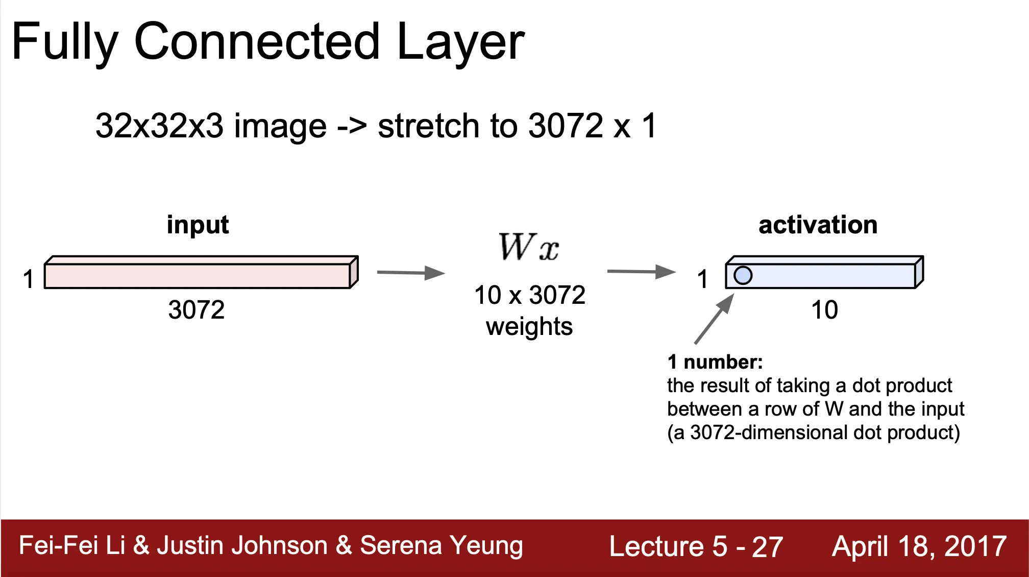
Input 은 1 dimensional vector (N×1N\times 1N×1)

◦

만약 Input 전 단계에서 3 dimensional vector 가 산출 되었다면 1 dimensional vector 로 flatten 하는 과정이 필요

•

Weight 는 2 dimensional vector (M×NM\times NM×N)

•

Output 은 1 dimensional vector - activation (M×1M\times 1M×1)

•

연산 자체는 matrix multiplication 과 동일

◦

activation=Wx\rm{activation}=\it{Wx}activation=Wx

•

Convolutional Neural Network 의 끝에 와 이때까지 구했던 vector 와 모두 연결된 새로운 vector 를 만들어내는 역할 (inference 에 모든 input vector element 가 사용됨)

Convolution Layer

•

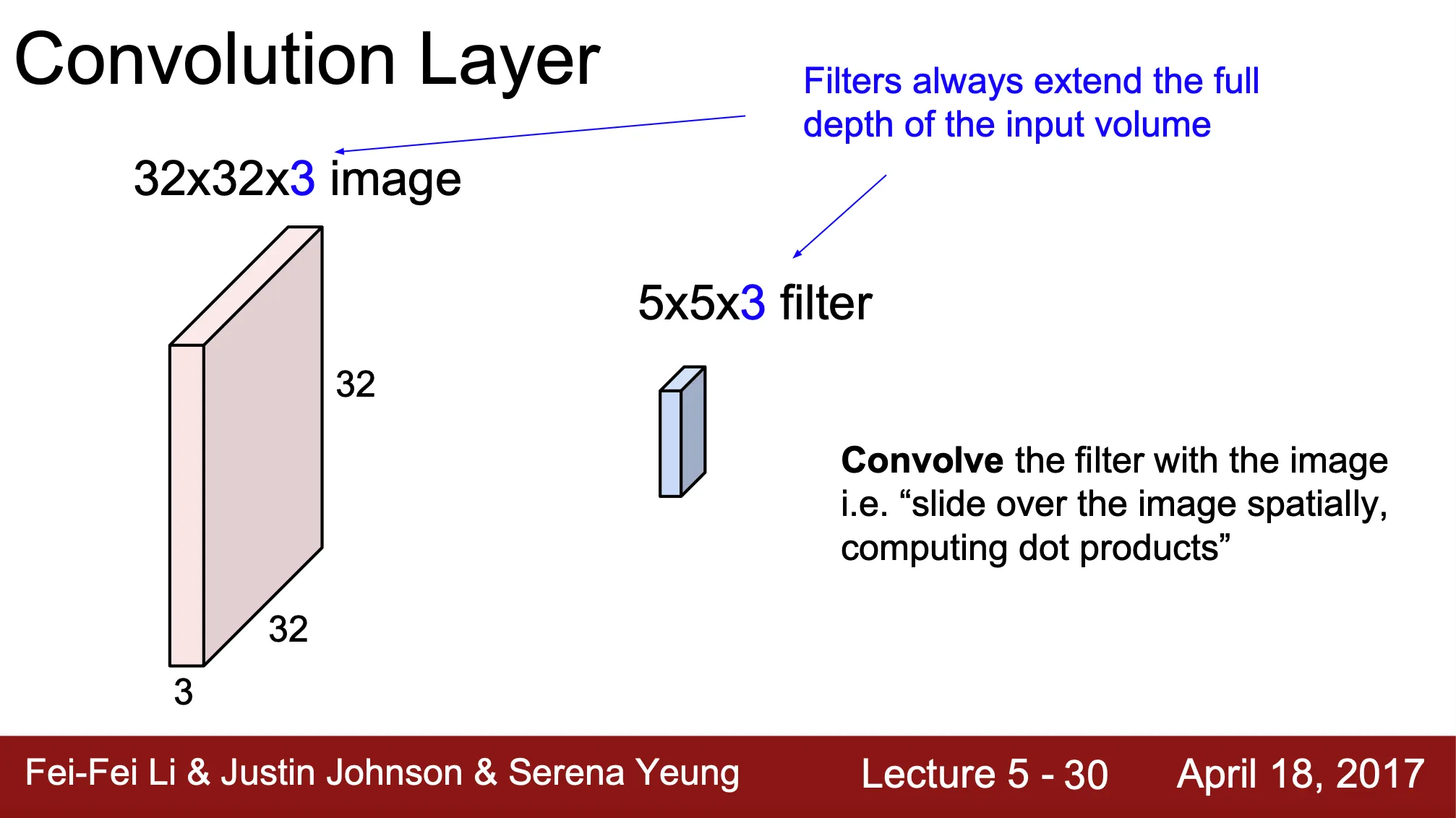
Fully Connected Layer 와는 다르게 spatial structure 를 유지

•

Image, 혹은 이전 단계의 vector 를 convolving 하는 filter 가 존재

◦

filter = kernel = receptive field 모두 혼용해서 사용하는 단어

◦

filter 는 convolution layer 에서의 weight

•

Filter 가 image 를 convolve 하면서 spatial region 만큼을 dot product 한 값을 산출하여 새로운 output vector 를 산출 (이를 위해서는 image 와 filter 의 depth 가 같아야 함)

◦

위 사진의 예시로는, 두 image 가 겹치게 되었을 때 서로 겹치는 부분을 곱해서 나온 값을 서로 다 더해서 새로운 값 하나를 뽑아내는 것임 (Sum of Product)

◦

새로운 값 하나를 뽑아내는 과정을 image 를 convolve 하면서 계속 진행해서 spatial structure 가 유지된 새로운 output vector 를 산출

◦

한 칸씩 이동하며 convolving 할 경우, 28×28×128\times28\times128×28×1 의 output vector 가 생성

•

Filter 의 개수만큼 output vector 의 depth 가 증가 (위에 설명한 과정을 filter 의 개수만큼 반복해서 쌓아가는 형태)

•

Convolution 연산?

◦

image 에 padding 이 붙은 새로운 vector 위를 filter 가 stride 만큼씩 이동하며 convolve 하여 output vector 를 산출

◦

stride: filter 가 image 를 convolve 할 때 filter 가 한 번에 이동하는 pixel 수

◦

padding: image 의 가장자리에 붙는 zero-padding 의 두께 pixel 수

◦

pp p 만큼의 padding 을 가지는 N×NN\times NN×N image 위를 F×FF\times FF×F filter 가 sss 만큼의 stride 를 가진채 convolve 할 경우 output vector 의 spatial dimension 은?

▪

[(N−F+2×p)/s+1]×[(N−F+2×p)/s+1][(N-F+2\times p)/s + 1] \times [(N-F+2\times p)/s + 1][(N−F+2×p)/s+1]×[(N−F+2×p)/s+1]

▪

example 1) Output Dimension?
1. Input dimension: 32×32×332\times32\times332×32×3
2. 10 5×5\rm{10}\ 5\times510 5×5 filters
3. stride 1
4. padding 2
→ (32−5+2×2)/1+1=32(32-5+2\times2)/1 +1=32(32−5+2×2)/1+1=32
→ 32×32×1032\times32\times1032×32×10

▪

example 2) Parameter Number?
1. Input dimension: 32×32×332\times32\times332×32×3
2. 10 5×5\rm{10}\ 5\times510 5×5 filters
3. stride 1
4. padding 2
→ (5×5×3(input depth)×+1(bias))×10(# filter)=760(5\times5\times3(\rm{input \ depth})\times+1(\rm{bias}))\times10(\rm{\#\ filter})=760(5×5×3(input depth)×+1(bias))×10(# filter)=760

Pooling Layer

•

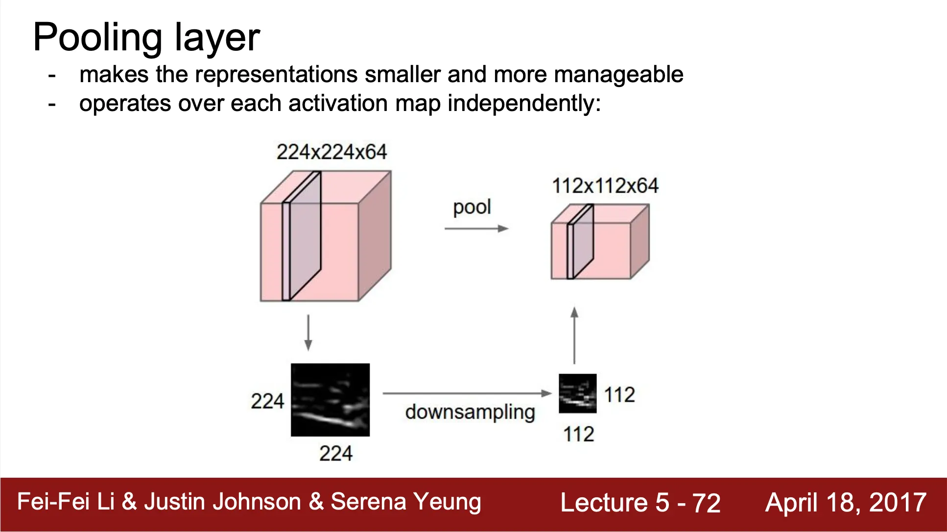
Representation 을 더 작은 dimension 으로 변환하는 역할 (downsampling)

•

오로지 spatial dimension 만을 downsample

•

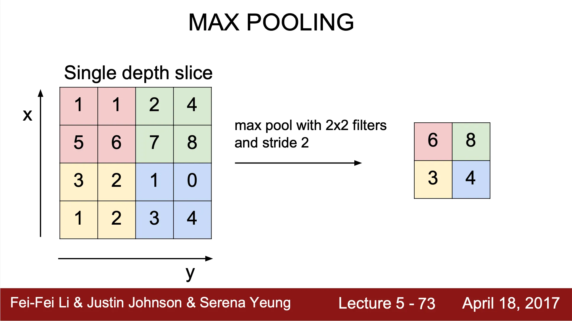
Max Pooling 연산?

◦

filter size 내에서 가장 큰 값을 산출하여 대표 값으로 설정

◦

Convolution Layer 처럼 filter 가 stride 만큼 움직이며 output value 를 산출하면서 reduced 된 형태의 spatial structure 를 만들어냄

◦

Convolution Layer 와 다르게 padding 이 존재하지 않음

•

input image W1×H1×D1W_1\times H_1\times D_1W1​×H1​×D1​ 를 F×FF\times FF×F 의 filter 가 stride sss 를 가지면서 pooling 하여 W2×H2×D2W_2\times H_2\times D_2W2​×H2​×D2​ 가 산출되었을 때, 

W2=(W1−F)/s+1W_2=(W_1-F)/s +1W2​=(W1​−F)/s+1
H2=(H1−F)/s+1H_2=(H_1-F)/s +1H2​=(H1​−F)/s+1
D2=D1D_2=D_1D2​=D1​

를 가짐. Convolution Layer 와 동일하지만, padding ppp 만 존재하지 않음.

Convolutional Neural Network 의 heirarchy

•

Convolutional Layer + ReLU 가 층층히 쌓여 있고, 마지막에 Fully Connected Layer + SoftMax

•

각 층마다 나타나는 feature 의 형태가 다름

◦

Low-level: Low-level features, edges

◦

Middle-level: Middle-level features, corner & blobs

◦

High-level: High-level features, resembled blobs

•

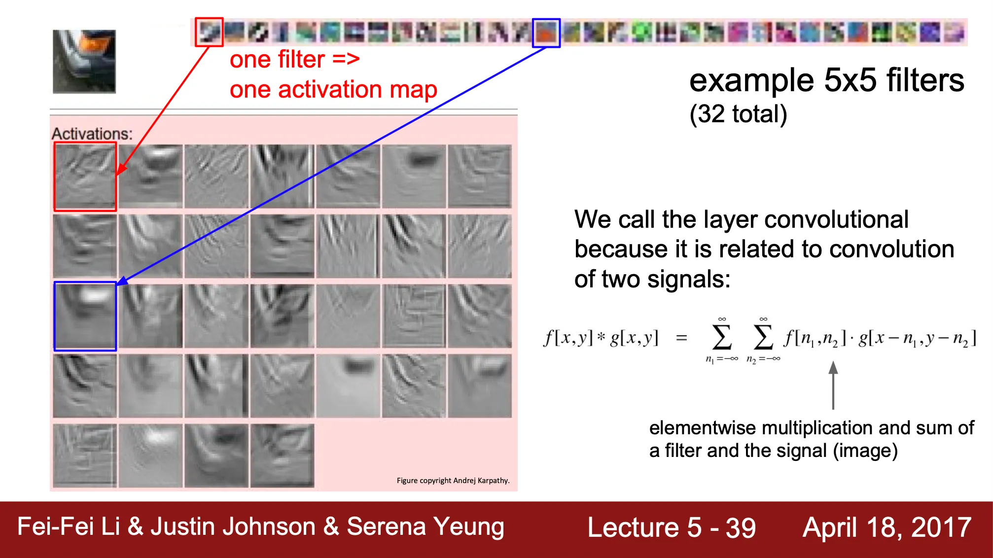
각 filter 가 관찰하는 이미지의 특성이 다르고, 이것이 actiavation map 에 드러남

◦

각 filter 의 형태 (template) 이 이미지에서 어떻게 나타나는가가 dot product 결과인 activation map 에 드러남

◦

붉은 박스의 filter 의 activation map 은 자동차 전조등의 edge 를 잘 관찰해냄