Lecture 3 | Loss Functions and Optimization

포스팅 날짜

2021/07/15

지난 강의 보기 - Lecture 2 | Image Classification

다음 강의 보기 - Lecture 4 | Introduction to Neural Network

Note Taking

Lecture 2 요약

•

Recognition 이 어려운 이유 ?

◦

컴퓨터가 보는 데이터와 실제 보는 시각의 큰 차이..

◦

Illumination

◦

Deformation

◦

Occlusion

◦

Clutter

◦

Intraclass Variation

•

K-Nearest Neighborhood

◦

Cross Validation

◦

Setting Hyperparameter

•

Linear Classifier

◦

Parametric Approach (W)W)W)

Linear Classifier, 어떤 W 를 선택해야 할까 ?

•

Prediction (yi=Wxi)y_i=Wx_i)yi​=Wxi​) 의 결과로 옳은 class 의 score 를 제일 높게 뽑은 친구?

•

Prediction (yi=Wxi)y_i=Wx_i)yi​=Wxi​) 의 결과로 옳지 않은 class 의 score 를 낮게 뽑은 친구?

•

...

•

W 선택에 대한 정량적인 기준이 필요

Loss

•

W 선택에 대한 정량적인 기준

•

얼마나 W 가 좋지 않은가 (How badness the loss is)

•

LiL_iLi​: individual data 에 대한 loss

•

LLL: ∑i=1i=NLi\sum_{i=1}^{i=N} L_i∑i=1i=N​Li​,  whole data 에 대한 loss

Classifier 에 사용할 수 있는 Loss

•

Multiclass SVM Loss

L_i=\sum_{j\neq y_i}\max({0, s_j-s_{y_i}+1})

Correct class 의 score 가 Incorrect class 의 score 에 배해서 일정한 margin 이상 높다면 penalize 하지 않고, 그렇지 않다면 margin 에서 부족한 정도만큼 penalize 하기 위한 설계

◦

Hinge Loss 라고도 함

◦

Minimum: 0, Maximum: Infinity

◦

sjs_jsj​ 들이 모두 같은 경우: Li:#Number of Classes−1L_i: \mathrm{\#Number\ of\ Classes} -1Li​:#Number of Classes−1

◦

합에 j=yij=y_ij=yi​ (correct class 에 대한 loss) 도 포함된다면 LiL_iLi​ 는 1 만큼 커짐

◦

합에 j=yij=y_ij=yi​ (correct class 에 대한 loss) 도 포함한 식으로 사용해도 무방하나 minimum value 를 0 으로 만들기 위해서 보통은 포함하지 않음

◦

합 대신 평균 식을 사용해도 무관 (Rescaling)

◦

Zero loss 가 나타나는 W0W_0W0​ 는 non-unique (ex. 2W02W_02W0​)

•

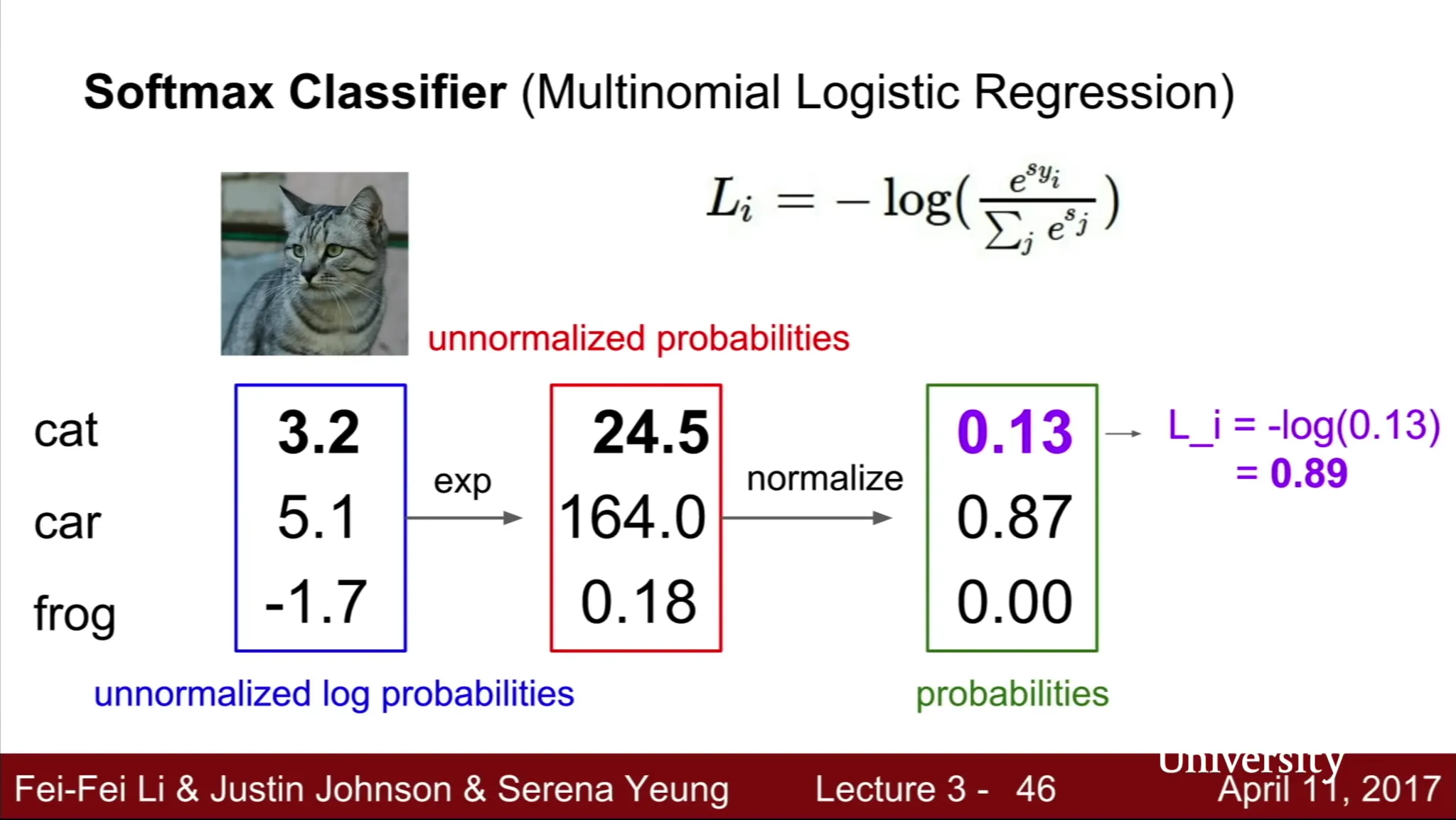
Softmax Loss

L_i=-\log{P(Y=y_i|X=x_i)}=-\log(\frac{e^{s_{y_i}}}{\sum_j e^{s_j}})

Multiclass SVM Loss 의 score 는 의미를 가지지 않는데 비해 Sofmax 는 각 class 일 확률의 unnormalized log 형태

◦

zero loss 가 나오려면 correct class score 는 infinity, incorrect class score 는 minus infinity 가 되어야 하기 때문에 실질적으로 실제 상황에서 나올 수는 없음

◦

W 가 초기에 매우 작아 모든 score 가 0 에 가깝다면 첫 loss 는 −log⁡(1#Number of Classes)=log⁡(#Number of Classes)-\log(\frac{1}{{\mathrm{\# Number\ of \ Classes}}})=\log({\mathrm{\# Number\ of \ Classes}})−log(#Number of Classes1​)=log(#Number of Classes)

•

SVM loss VS Softmax loss

SVM loss 는 0 지점에서 correct score 의 jiggling 이 일어나더라도 loss 의 변화가 없는 반면, Softmax 는 계속해서 correct score 의 크기를 크게, incorrect class score 를 작게하려는 차이가 있음

Regularization

•

Loss 가 낮은 W 를 선택하는 것은 좋으나 training data loss 보다는 test data loss 가 훨씬 중요함

•

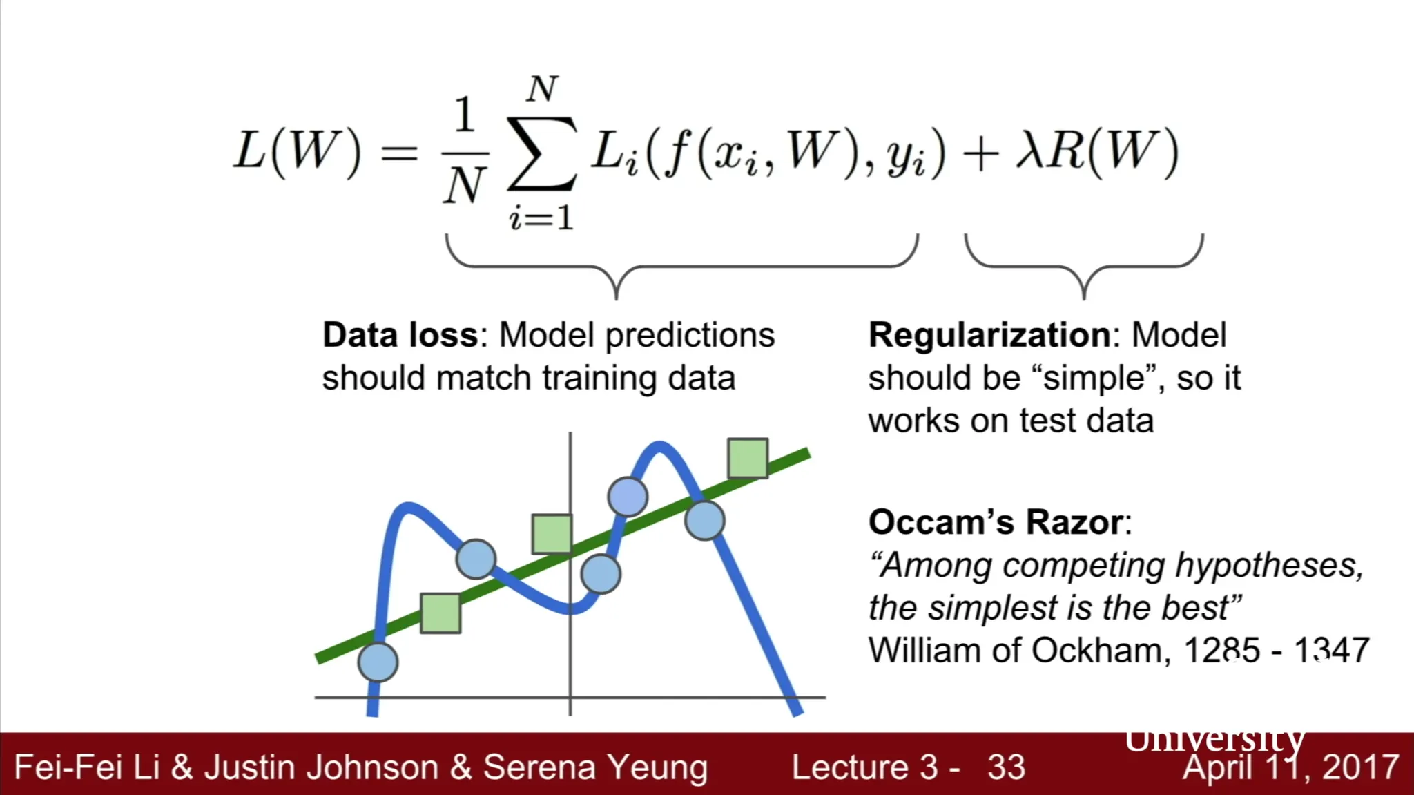
Loss 가 실패하는 원인 중 하나: 높은 Model 의 복잡도 

•

Regularization loss term 을 두어 model 을 simple 하게 만듬. 

•

λ\lambdaλ: Hyperparameter, data loss 와 regularization loss 의 가중치 조절

Regularization 종류

•

L2 Regularization

◦

R(W)=∑k∑lWk,l2R(W)=\sum_k\sum_lW_{k,l}^2R(W)=∑k​∑l​Wk,l2​

◦

L2 Regularization 이 complex model 을 penalize 하는 이유?

▪

W 의 각 요소들이 가지는 influence 를 전체적으로 퍼뜨리는 효과 
하나의 튀는 값을 가지게 하지 않으며 parameteric function 을 전반적으로 smooth 하게 만듬

•

L1 Regularization

◦

R(W)=∑k∑l∣Wk,l∣R(W)=\sum_k\sum_l \left| W_{k,l}\right|R(W)=∑k​∑l​∣Wk,l​∣

•

Elastic Net Regularization

◦

L2, L1 Regularization 을 합친 형태 (with constant β\betaβ)

◦

R(W)=∑k∑lβWk,l2+∣Wk,l∣R(W)=\sum_k\sum_l \beta W_{k,l}^2 + \left| W_{k,l}\right|R(W)=∑k​∑l​βWk,l2​+∣Wk,l​∣

•

Max Norm Regularization

•

Dropout

•

Fancier: Batch Normalization, Stochastic Depth (in deep learning)

Optimization

•

Loss 를 최소화하는 방법

•

Random Search

◦

W 를 잔뜩 유추하고 그것에 대한 loss 를 구해봄

•

 Follow ths Slope

◦

Negative Gradient Vector Direction

◦

Numerical Gradient: Approximate, Slow, Easy to write

◦

Analytic Gradient: Exact, Fast, Error-prone

◦

Gradient Descent !

▪

Initialize Weight

▪

While true, compute loss and gradient to update weight in minus gradient direction

▪

Step size, Learning rate: hyperparameter

•

Ex. Stochastic Gradient Descent

L(W) = \frac{1}{N}\sum_{i=1}^{i=n}L_i(f(x_i,W),y_i) +\lambda R(W)

\nabla_WL(W)=\frac{1}{N}\sum_{i=1}^{i=n}\nabla_WL_i(f(x_i,W),y_i) +\lambda \nabla_WR(W)

전체 dataset 을 가지고 loss 를 구하고, gradient 를 계산한 후 weight 를 update 하면 느림 ㅜㅜ

Mini-batch 를 사용하여 일부 dataset 을 사용한 loss 를 구하고 전체 loss 를 estimate 한 후 update

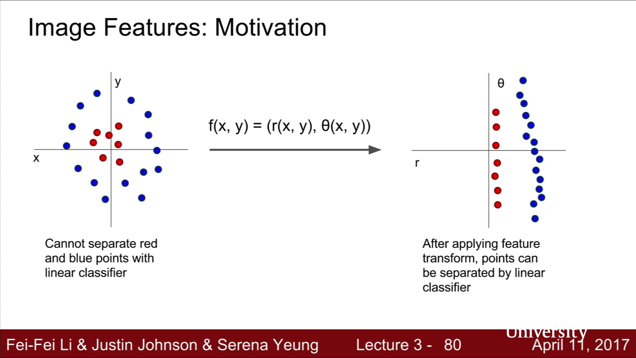
Aside: Image Feature

•

Raw pixel value 를 그대로 classifier 에 넣는 것은 제대로 동작하지 않을 때가 많음

•

기존의 classifier 단계에 feature extraction 을 추가

•

Ex. Color Histogram

◦

이미지의 각 픽셀을 color 에 따라 나누어 color historgram 으로 나눔

◦

Color Historgram 자체가 feature

•

Ex. Histogram of Oriented Gradients (HoG)

◦

Hubel and Wiesel 은 oriented edge 가 human visual system 에서 recognition 에 중요한 역할을 함을 알아냄

◦

Oriented Gradient 에 대한 feature representation 은 edge 의 local orientation 을 대변

◦

각 8x8 pixel 마다 9 개의 방향성을 부여 → 320x240 image 는 40x30 bin 을 가지고 각 bin 당 9 개의 direction 을 가지므로 30x40x9 feature vector 가 생김

•

Ex. Bag of Words

◦

Build Codebook

▪

Random Patches 를 image 로부터 뽑아서 Clustering Center 가 될 codebook 을 형성

◦

Encode Images

▪

이미지를 만든 codebook 에 따라 clustering 하여 (encode) 각 visual word 가 얼마나 등장하는지에 대한 histogram 을 만들 수 있음

최종적으로 Image Classification Pipeline 은

Input Image

Feature Extraction (학습되는 부분이 아님)

ConvNets (학습되는 부분)

로 구성되어 있다고 볼 수 있음