Lecture 7 | Training Neural Networks (2)

포스팅 날짜

2021/08/13

지난 강의 보기 - Lecture 6 | Training Neural Networks (1)

다음 강의 보기 - Lecture 8 | Deep Learning Software

Note Taking

Lecture 6 요약

•

Activation Functions

◦

Sigmoid - Not Zero-Cenetered, Saturation

◦

tanh - Zero-Cenetered, Saturation

◦

ReLU - Half-region Saturation, Not Zero-Centered

◦

Leaky ReLU & Parametric ReLU - Partially Zero-Centered, Non-Saturation

◦

ELU - Partially Zero-Centered, Half-region Saturation

◦

Maxout - Layer Approach of giving non-linearity

•

Weight Initialization

◦

Zero Initialization - Update symmetrically

◦

Small Standard Normal Initialization - Activation falls into 0

◦

Big Standard Normal Initialization - Activation falls into -1, 1

◦

Xavier Initialization - Regualte activation to follow normal distribution

◦

He Initialization - Cosider ReLU activation function (which kills half of neuron activation)

•

Batch Normalization

◦

Activation 이 Normal distribution 을 따르게 하고 싶으면 그렇게 만들어주면 되잖아?

◦

Batch 속 이미지들의 mean 과 variance 를 계산하여 training time 에 normalize

•

Hyperparameter Optimization

◦

Coarse to Fine Cross-Validation

Optimiazation

•

Stochastic Gradient Descent (SGD)

◦

가장 일반적인 optimiazation

◦

전체 dataset 에 대한 loss 를 구한 뒤 update

◦

Mini-batch Gradient Descent 의 변종 존재

•

SGD + Momentum

◦

SGD 는 local minima 나 saddle point 에 갇히는 문제가 존재

◦

Feature 마다 다른 scale 의 gradient 를 가진다면, 비효율적인 optimization 이 진행

◦

Gradient 에 관성적인 요소를 더해 이전의 gradient dependent 한 gradient 를 산출

◦

vt+1=ρvt+∇f(xt)xt+1=xt−αvt+1v_{t+1}=\rho v_t+\nabla f(x_t)\\
x_{t+1}=x_t-\alpha v_{t+1}vt+1​=ρvt​+∇f(xt​)xt+1​=xt​−αvt+1​

◦

강의에서는 위 표기를 썼지만, 일반적으로는
vt+1=ρvt−α∇f(xt)xt+1=xt+vt+1v_{t+1}=\rho v_t-\alpha\nabla f(x_t)\\
x_{t+1}=x_t+v_{t+1}vt+1​=ρvt​−α∇f(xt​)xt+1​=xt​+vt+1​
의 형태로 적음 (intuition 만 이해하고 넘어가도 될 듯함)

◦

vtv_tvt​ 는 velocity 를 대변하는 요소로, gradient 와 dimension 이 같음

◦

전 step 의 velocity 를 ρ\rhoρ 만큼의 fraction 으로 현재 step 에서 반영함

•

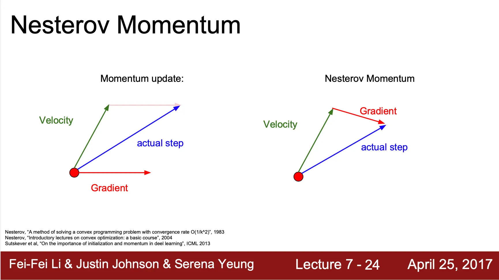
Nesterov Momentum

◦

SGD + Momentum 이 과거의 gradient 를 반영했다면, Nesterov Momentum 은 미래의 위치에서의 gradient 도 현재 step 에서 함께 반영하여 학습 속도의 증가를 기대함

◦

vt+1=ρvt−α∇f(xt+ρvt)xt+1=xt+vt+1v_{t+1}=\rho v_t-\alpha\nabla f(x_t+\rho v_t)\\
x_{t+1}=x_t+v_{t+1}vt+1​=ρvt​−α∇f(xt​+ρvt​)xt+1​=xt​+vt+1​

◦

vt+1v_{t+1}vt+1​ 를 계산할 때 현재 위치에서 현재 vtv_tvt​ 만큼 지속된다고 가정하고 이동한 위치에서의 gradient 를 이용해 계산

•

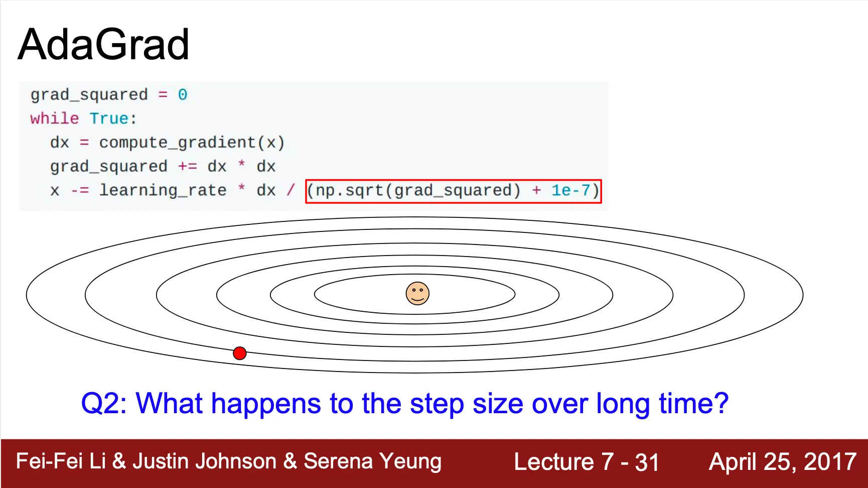
AdaGrad

◦

앞의 optimization algorithm 들이 가졌던 elementwise gradient scaling 문제를 해결

◦

각 weight element 마다 지금까지 update 된 정도를 기반으로 수렴 정도를 판단해 현재 update 의 정도를 정함

◦

Update 시 마다 grad_squared 에 gradient 의 squared 값을 더해서 가지고 있다가, 현재 step 에서 그 값의 squared root 로 나눠줌

◦

초기 0 으로 나누는 것을 방지하기 위해 bias term 을 둠 (아래 그림에서의 1e−71e-71e−7)

•

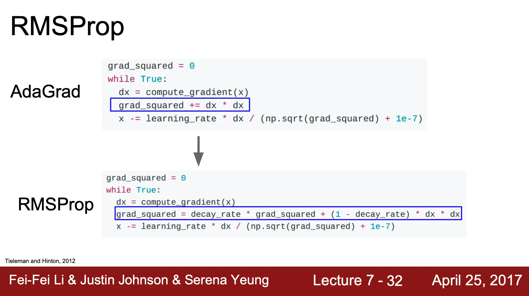
RMSProp

◦

당연하게도, AdaGrad 는 시간이 갈 수록 (Update 횟수가 많아질 수록) update 하는 scale 이 점점 작아졌고, 결국 update 잘 일어나지 않게 되는 현상이 발생

◦

누적하는 항목인 grad_squared 에 exponential decaying average 를 적용하여 과거의 gradient 일 수록 현재의 gradient 산출에 굉장히 작은 영향을 주도록 변경

•

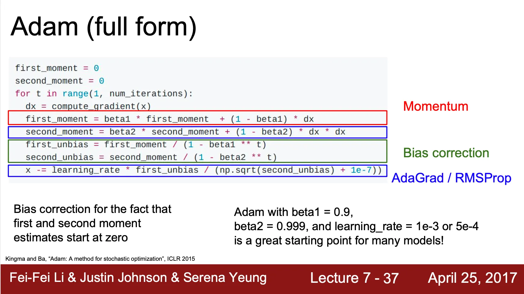
Adam

◦

Momentum 과 RMSProp 가 합쳐진 형태의 optimization algorithm

◦

기존의 momentum 은 ρ\rhoρ 의 항목으로 이전의 gradient 를 반영한다고만 했는데, Adam 에서는 앞의 RMSProp 처럼 exponential decaying average 를 적용한 first momentum 이라는 값으로 바꿈

◦

기존 RMSProp 에서 명시했던 grad_squared term 은 second momentum 으로 명시

◦

xt+1=xt−α×first momentum/second momentum+biasx_{t+1} = x_t - \alpha\times\rm{first\ momentum}/\sqrt{second\ momentum + bias}xt+1​=xt​−α×first momentum/second momentum+bias​

◦

그러나, 보통 아래 그림에서의 β1\beta_1β1​, β2\beta_2β2​ 는 1 에 가까운 값으로 관성적 요소가 크게 설정하는데 설상가상으로 초기 first momentum 과 second momentum 의 설정이 0 이기 때문에 초기 각 momentum 은 값이 작음

◦

이 때, 초기에 보여지는 update 가 굉장히 큰데, 이를 막기 위해 bias correction 과정을 진행 (초기에만 momentum 을 크게 만들어주는 역할을 함)

◦

first unbias=first momentum1−β1t\rm{first\ unbias} = \frac{first\ momentum}{1-\beta_1^t}
first unbias=1−β1t​first momentum​
second unbias=second momentum1−β2t\rm{second\ unbias} = \frac{second\ momentum}{1-\beta_2^t}
second unbias=1−β2t​second momentum​

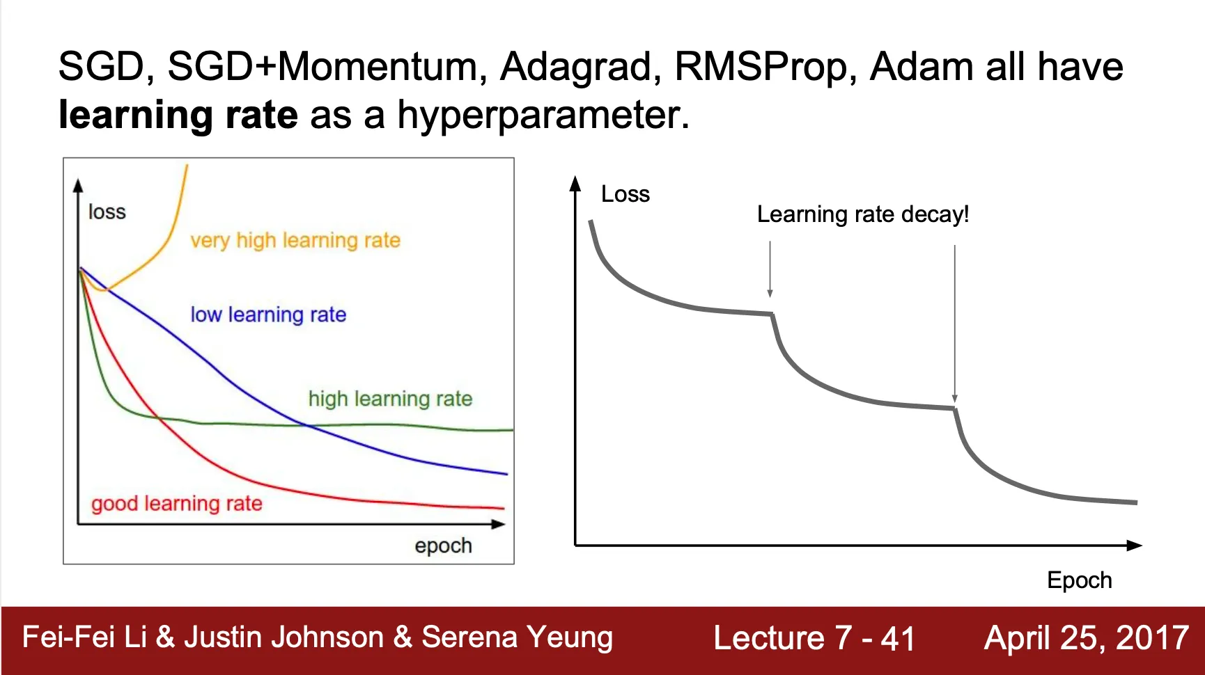
Learning Rate Schedule

•

SGD, SGD+Momentum, AdaGrad, RMSProp, Adam 모두 learning rate 항목을 가짐

•

Learning rate 는 수렴에 가까워질수록 작아지는 것이 수렴에 더 도움이 됨

•

Learning rate scheduling 

◦

Step decay
일정 epoch 이 지난 뒤에 일정 비율만큼 learning rate 감소

◦

Exponential decay
α=α0e−kt\alpha = \alpha_0e^{-kt}α=α0​e−kt

◦

1t\frac{1}{t}t1​ decay
α=α01+kt\alpha=\frac{\alpha_0}{1+kt}α=1+ktα0​​

•

Learning rate decay 는 second-order parameter 로 이를 처음부터 optimize 하는 것이 아님. Learning rate 를 정한 뒤에 cross-validation 을 진행하는 형태가 되어야 함.

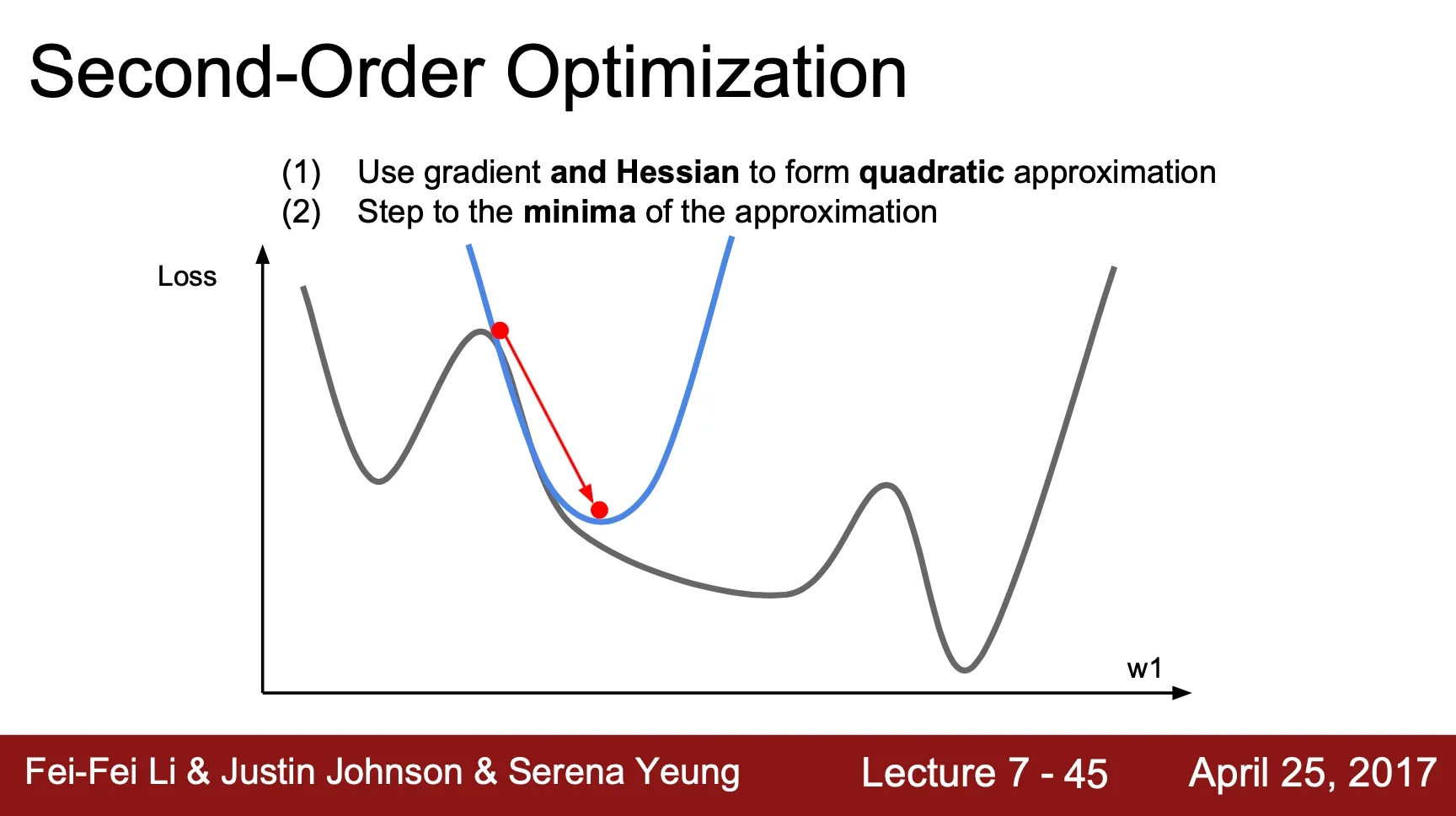
Second-Order Optimization

•

지금까지의 optimization 은 gradient 방향으로 learning rate step 만큼 이동하는, first-order optimization

•

Gradient 와 Hessian 을 모두 이용해 특정 지점의 quadratic approximation 을 구할 수 있고, 그 approximation 의 최솟값을 선택하는 형태의 optimization 방법론도 가능

•

Learning rate 필요 없이 update 가 최솟값으로의 이동을 나타냄

•

Hessian 을 계산하는 것이 굉장히 expansive 하여 실제 딥러닝에서는 효과적이지 못함

◦

Quasi-Newton method (BFGS 등) 를 사용해 inverse Hessian 을 근사하여 계산할 수 있음

◦

Full inverse Hessian 을 저장하지 않는 L-BFGS 를 사용하는 것은 고려할만한 선택지

Model Ensembles

•

여러 개의 모델을 training 하여 test time 때 각각의 산출 값을 평균을 내는 방법

•

보통 약 ~2% 정도의 performance 개선이 일어남

•

ImageNet competition 같은 곳에서는 단골 손님

•

여러 개의 모델이 아닌, 한 모델의 training 중간 상태의 snapshot 을 기반으로 ensemble 을 할 수도 있음

◦

Learning rate 를 높였다 낮췄다 하면서 모델의 수렴점을 다르게 바꿔가면서 snapshot 을 따고 ensemble 하는 crazy 한 방법도 존재

•

Polyak Averaging

◦

각 neuron 에서 exponential decaying average 를 꾸준히 계산하여 이를 inference time 에 사용

◦

간접적인 ensemble 효과를 불러옴

Regularization

•

Training set 에 overfit 된 single model 의 peformance 를 늘리는 방법

•

L1 Regualrization

◦

Weight

◦

R(W)=∑k∑l∣Wk,l∣R(W)=\sum_k\sum_l\left|W_{k,l} \right|R(W)=∑k​∑l​∣Wk,l​∣

•

L2 Regularization

◦

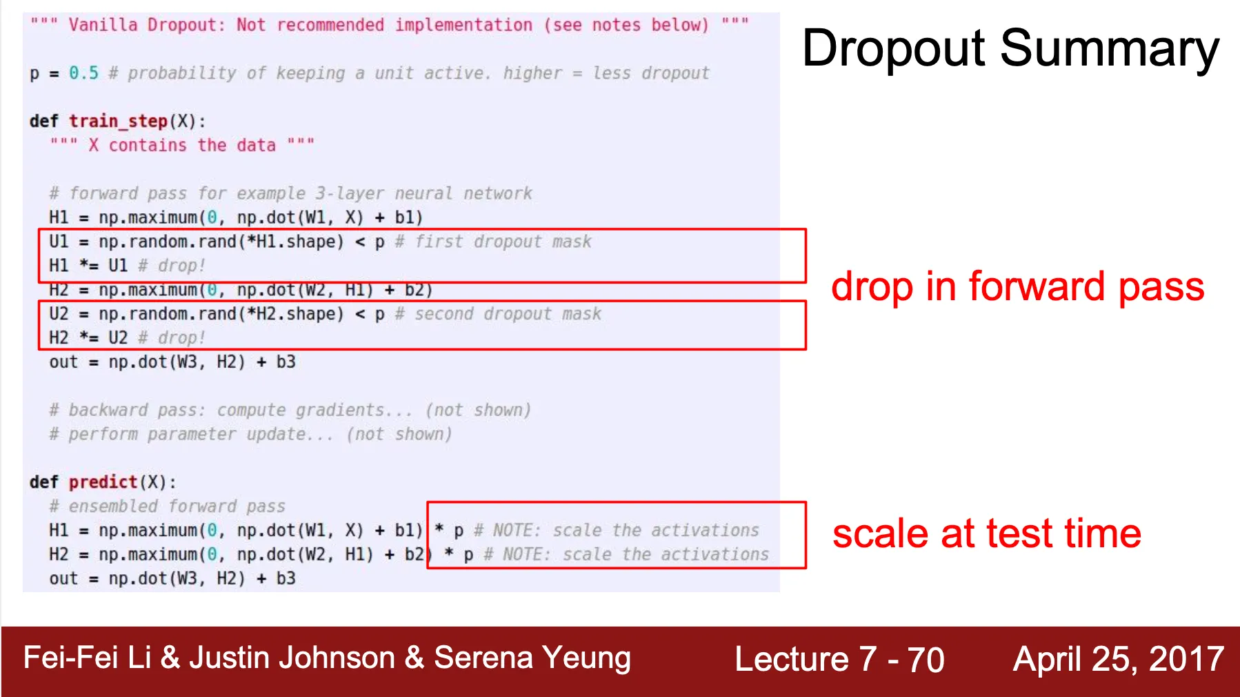
R(W)=∑k∑lβWk,l2+∣Wk,l∣R(W)=\sum_k\sum_l\beta W_{k,l}^2+\left| W_{k,l} \right|R(W)=∑k​∑l​βWk,l2​+∣Wk,l​∣

•

Dropout

◦

Training 단에서 모델의 복잡도를 줄이는 방법론

◦

Forward propagation 과정에서 neuron 의 activation 을 0 으로 만들어 모델 구조 상의 연결 관계를 해제하는 기법

◦

Hyperparameter 인 probability ppp 를 기반으로 activation 을 0 으로 만들 비율을 설정

◦

Activation 이 random 하게 0 이 된 굉장히 많은 형태의 네트워크의 ensemble 로 볼 수도 있음

◦

하나의 특성에 너무 과도하게 집중하는 형태를 방지하기 때문에 좋은 효과를 보임 

◦

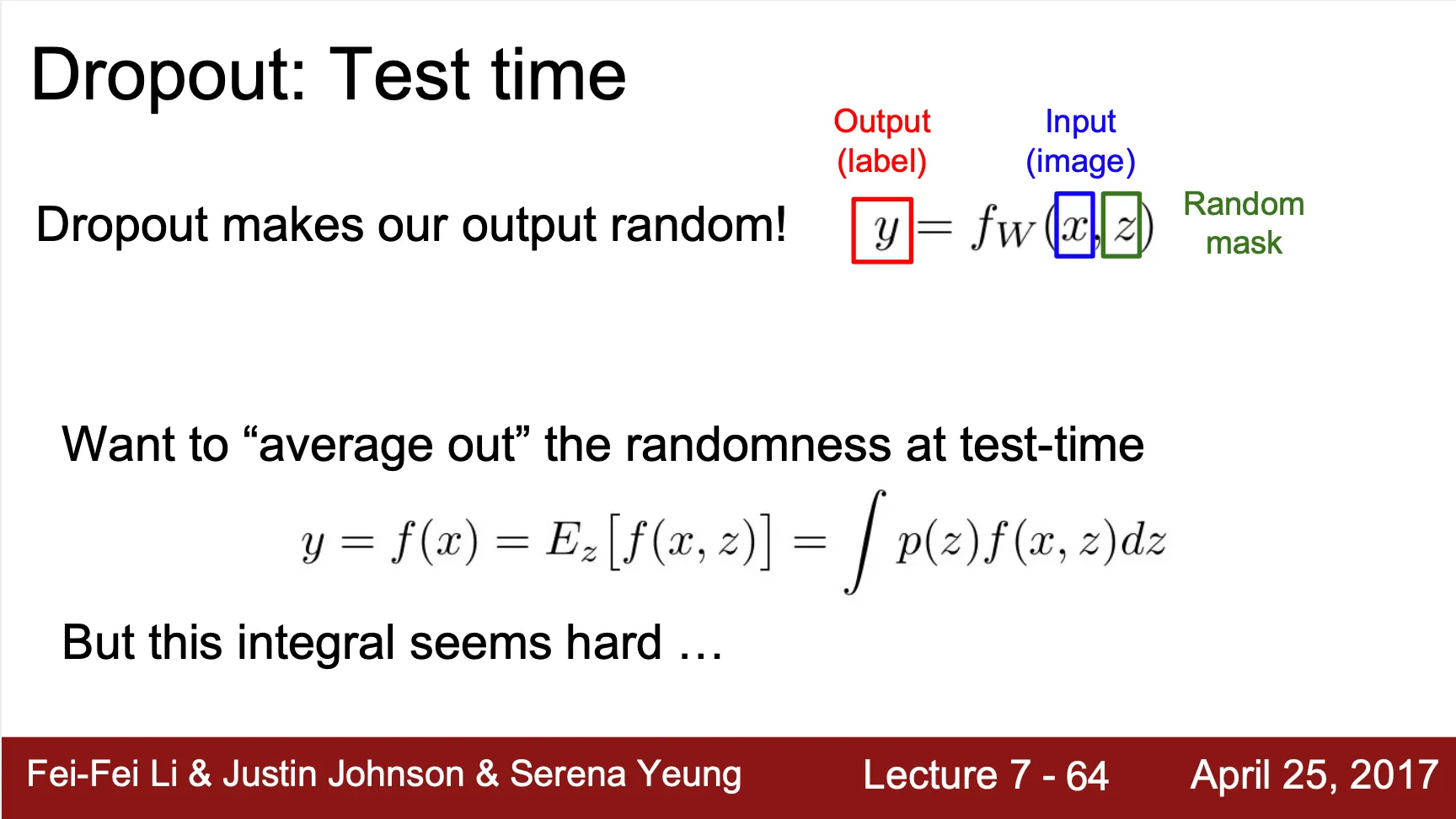
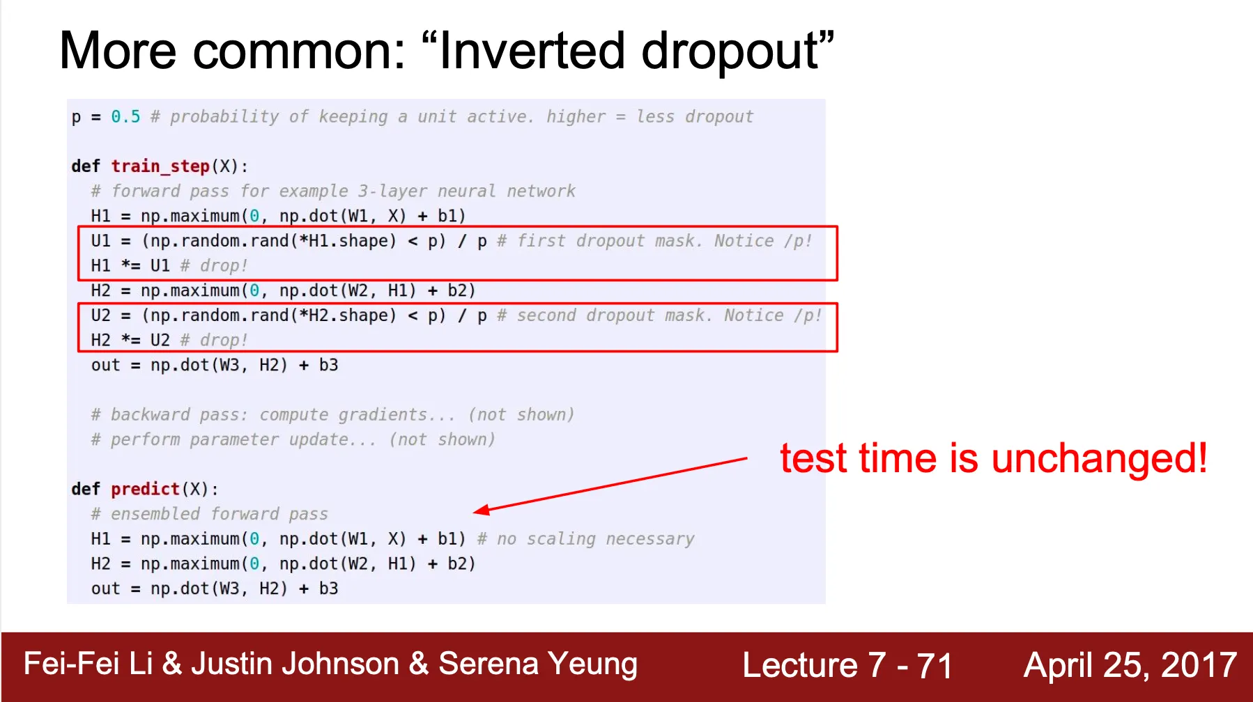
Inference time 에도 dropout 을 적용하게 되면 random mask 가 포함된 output 이 나오기 때문에 inference 를 할 때마다 결과가 달라짐

▪

하지만, random mask 를 포함한 결과를 모두 다 integration 하기에는 intractable 함

▪

때문에, inference time 에는 결과에 dropout probability, ppp 를 곱하는 형태의 local, cheap approximation 을 진행

▪

Inference time 에서는 효율성이 중요하기 때문에 training time 에 오히려 Inverted dropout 이라 하여 1p\frac{1}{p}p1​ 를 곱하는 형태로 진행도 가능

•

Data Augmentation

◦

Data set 의 개수를 늘리는 방법론

◦

Horizontal Flips

▪

수평으로 이미지를 뒤집음

◦

Random crops & scales

◦

Color jitter

◦

Translation

◦

Rotation

◦

Stretching

◦

Shearing

◦

Lens distortions

•

DropConnect

◦

Training 단에서 모델의 복잡도를 줄이는 방법론

◦

Dropout 이 activation 을 0 으로 만드는 기법이라면, dropconnect 는 weight 를 0 으로 만드는 기법

•

Fractional Max Pooling

◦

Pooling 할 영역을 random 하게 지정하는 형태의 max pooling

•

Stochastic Depth

◦

Training 단에서 모델의 복잡도를 줄이는 방법론

◦

Forward propagation 과정에서 random 하게 layer block 을 끊고 이전의 layer block 의 결과를 가져와 학습하는 방법

Transfer Learning

•

Pre-trained model 을 사용하여 적은 데이터로도 모델을 학습하는 방법론

•

모델의 앞 부분의 weight 는 유지한 채로 끝 부분(Fully Connected Layer) 을 새로운 데이터에 맞게 변경 후 재학습

•

모델의 앞 부분의 feature 는 generality 가 큰 부분(Edge, Gabor Filter 등) 이므로 학습 데이터나 목적에 크 영향을 받지 않으나 모델의 뒷 부분의 feature 는 specificity 가 큰 부분(Blobs) 이므로 재학습이 필요