
Simple case: Translations
•
두 개의 parameter , 를 구하는 것
•
Correspondence Point 를 찾은 이로부터 , 를 구해내면 이미지를 matching 할 수 있음.
•
Mean Displacement of match
◦
Corresponding Point 간의 displacement 의 평균
•
하나의 Corresponding Point Pair 만 있어도 , 는 구할 수 있음.
◦
Paramter 2 개, Corresponding Point Pair 하나마다 2 개의 equation 이 나오기 때문임.
◦
보통의 경우에는 unkown 의 수보다 equation 이 많은 overdetermined system 을 구성하고 Least Square Solution 을 사용함
Least Squares Formulation
•
Translation Transform
◦
Squared Residual 의 합을 최소화하는 것을 목적으로 설정함
◦
위 식을 Matrix Formulation 으로 변경하여 구하면 다음과 같음.
▪
형태로 와 가 가져야 하면 좋을 값을 로 만든 형태임.
▪
이 최소화되는 를 찾는 것이 목표가 됨.
▪
미분해서 0 이 되도록 하는 값을 찾아봄
▪
보통은 역행렬을 구하는데 의 시간복잡도가 필요하기에 위 식의 역행렬을 구하지 않고, 많은 프로그램들이 제공하는 의 solver 를 사용함.
•
Affine Transform
◦
Residual & Cost Function 은 다음과 같음
◦
Matrix Formulation 으로 변경하면 다음과 같음.
•
Homography
◦
Homogeneous Coordinate 에서의 표현이므로 각 , 는 다음과 같음.
◦
Matrix Formulation 으로 변경하면 다음과 같음.
▪
Homography 에서는 특이하게 의 문제를 풀게 됨.
▪
는 up to scale 하므로 unit vector 에서만 문제를 해결하면 됨.
▪
8 unknowns → 4 개 이상의 Corresponding Points Pair 가 필요함.
▪
Solution: 는 의 smallest eigenvalue 를 가지는 eigenvector
Homography
•
Lagrangian Multiplier 를 도입하여 다음과 같이 쓸 수 있음.
•
minimize 를 위해 에 대한 derivative 이 0 인 를 구함.
◦
는 라는 eigenvalue 를 가지는 의 eigenvector
◦
이기 때문에 를 최소로 만드는 는 least eigenvalue 를 가지는 eigenvector 이고, 그 때의 값은 해당 eigenvalue 임. (Zero 일 수도 있음.)
Feature Matching
•
Mosaic 의 과정?
◦
Extract Interset Points (SIFT) → Unmatched Points 들로부터 matching 을 찾아냄 → Transformation 을 계산함
◦
많은 descriptor 사이의 match 를 찾는 과정이 Feature Matching
•
두 가지 방법론
◦
Exhaustive Search: 한 이미지의 feature 하나 당 다른 이미지의 모든 feature 를 순회하면서 비교해서 matching 되는 것들을 찾는, naive 한 방법론
◦
Nearest Neighbor Techniques: KD-tree 와 같은 tree 기반의 data structure 를 사용하면 neighereast neighbor 를 빠르게 찾을 수 있음.
•
Feature Matching 은 일반적으로 robust 하지 못하기 때문에 outlier 를 제거해내는 과정이 필요함.
Outliers
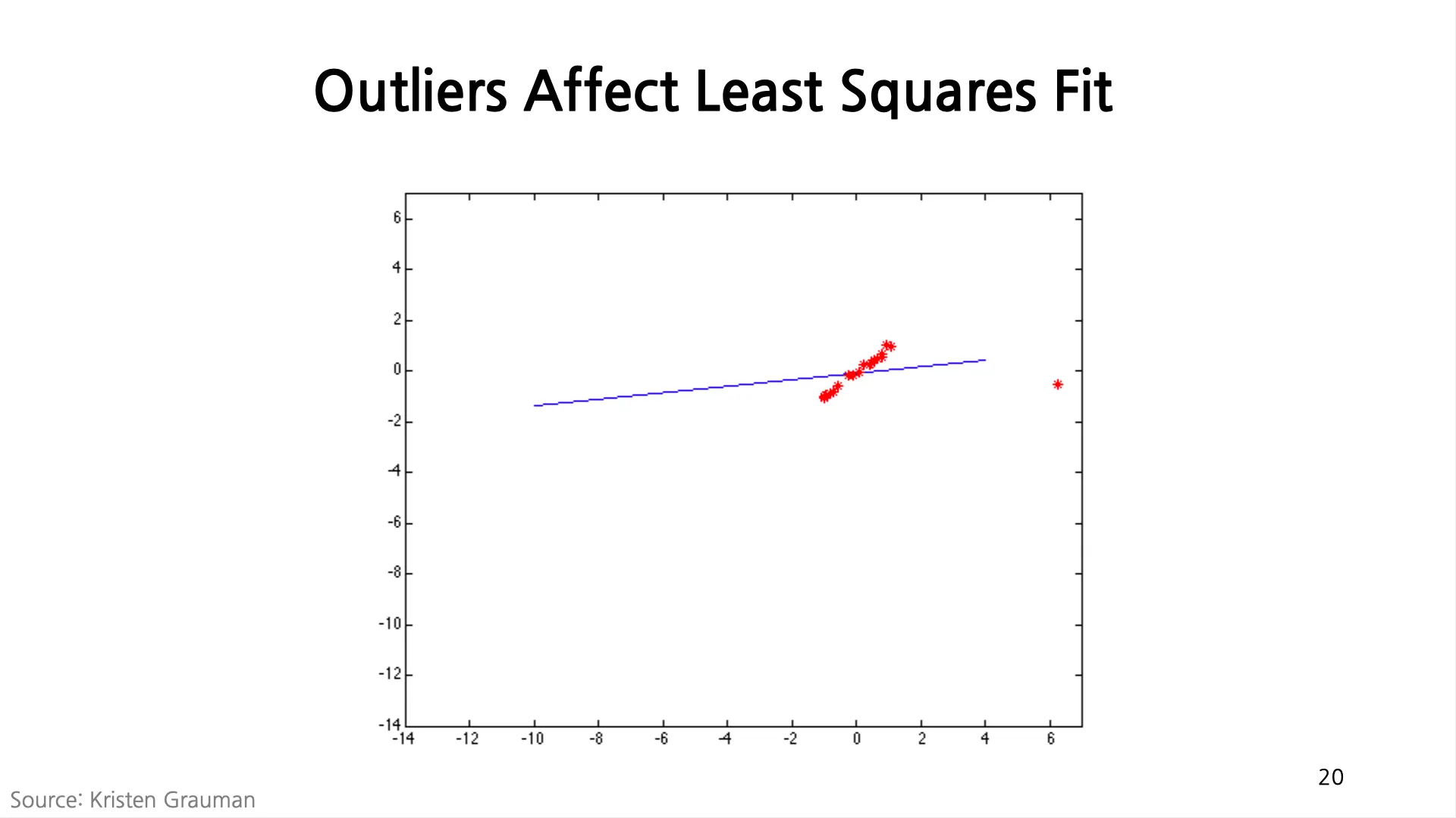
•
Outlier 는 Homography 의 parameter 를 예측하는데 있어서 그 성능을 크게 떨어뜨림
•
Wrong Match 를 제거하고 Correct Match 만을 이용해 Homography 를 계산하는 것이 중요함
RANSAC (RANdom SAmple Consensus)
•
Approach: Outlier 의 영향을 피해 Inlier 들만 사용하여 모델을 fitting 하려는 접근
•
Intuition: Outlier 가 현재의 fitting 을 계산하는데 사용되었다고 하면, 결과로 나오는 fitting 이 나머지 데이터들로부터 support 를 받지 못할 것이라는 직관에 기반
•
RANSAC loop
1.
랜덤하게 seed group of points 를 선택함
2.
Seed group of points 를 이용해 transformation 을 예측함
3.
찾은 transformation 에 부합하는 inlier 들을 찾아냄 (fitting 과의 error 가 threshold 보다 작은 친구들의 집합을 inlier 로 정의함.)
4.1. 찾아낸 inlier 의 수가 충분히 많으면, 해당 inlier 들을 모두 이용해서 다시 transformation 을 계산함
4.2. 찾아낸 inlier 의 수가 충분히 많지 않으면 1 번으로 돌아감.
RANSAC Example: Translation
1.
하나의 Corresponding Point Pair 를 랜덤하게 선택함.
2.
선택한 Corresponding Point Pair 를 이용해 transformation 을 구함.
3.
한 이미지의 점에 transformation 을 거쳐서 나온 점과 그 점의 corresponding point 과의 차이가 threshold 보다 작으면 inlier 로 취급하고, 전체 inlier 의 개수를 셈.
4.1. Inlier 의 개수가 충분히 많으면 해당 inlier 들을 모두 이용해서 다시 transformation 을 계산함.
4.2. Inlier 의 개수가 충분히 많지 않으면 1 번으로 돌아감.
RANSAC Pros and Cons
•
Pros
◦
Simple and General
◦
다양한 fitting 문제에 적용할 수 있음.
◦
현실에서도 잘 동작함.
•
Cons
◦
Seed Group 의 개수, Inlier 를 결정하기 위한 threshold, Inlier 가 충분히 많은지를 판단하기 위한 threshold 등 tuning 해야할 parameter 가 많음.
◦
Inlier ratio 가 낮으면 잘 동작하지 않음. (ex. 100 개의 matching 중 10 개만 실제로 correct matching 인 경우) → Keypoint Extraction 이나 Descriptor 를 바꾸는 것이 졸을 수도 있음.
◦
최소한의 개수를 이용해 transformation 을 초기에 구하는 것이 항상 좋은 initialization 이라고 보장할 수 없음.
Image Warping
•
RANSAC 으로 transformation 을 구했을 때, 해당 transformation 을 적용하여 변형한 이미지는 어떻게 변할 것인가를 알아내는 과정
•
Foward Warping, Inverse Warping 이 있는데, Inverse Warping 이 더 활용하기가 좋음.
•
Forward Warping
◦
원본 이미지로부터 시작해서 두 번째 이미지를 만들어내는 과정
◦
에 존재하는 픽셀 값을 대응되는 위치인 로 보내면 됨.
◦
하지만, 변환된 가 일반적으로 특정 픽셀에 딱 떨어지지 않음. → Splatting 근처의 픽셀에 색상을 배분해주는 과정을 활용함.
•
Inverse Warping
◦
변환된 두 번째 이미지로부터 원본 이미지를 재구성하려는 과정에서 나타나는 관계를 바탕으로 두 번째 이미지의 값들을 알아내는 과정
◦
의 각 픽셀에 를 적용하여 구해낸 원본 이미지의 위치의 픽셀값을 interpolation 으로 구해낼 수 있음. (값을 splatting 하는 것은 어렵지만 아는 값을 interpolation 하는 것은 쉬움.)
Bilinear Interpolation
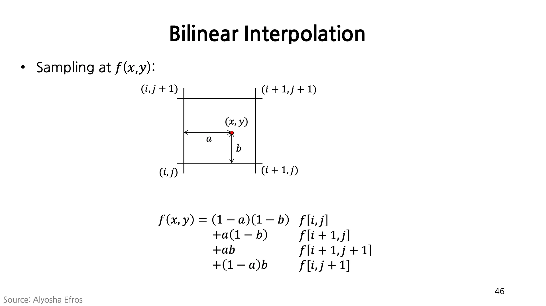
Image Warping with Homographies
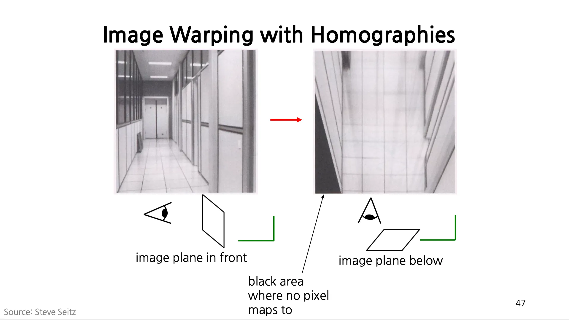
•
우측 그림의 검은색 영역은 Inverse Transformation 을 적용했을 때 원본 이미지의 범위 밖으로 나가서 표현될 수 없는 지역임.
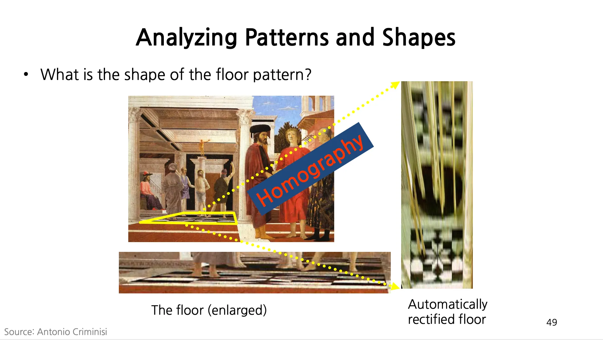
Image Rectificaiton
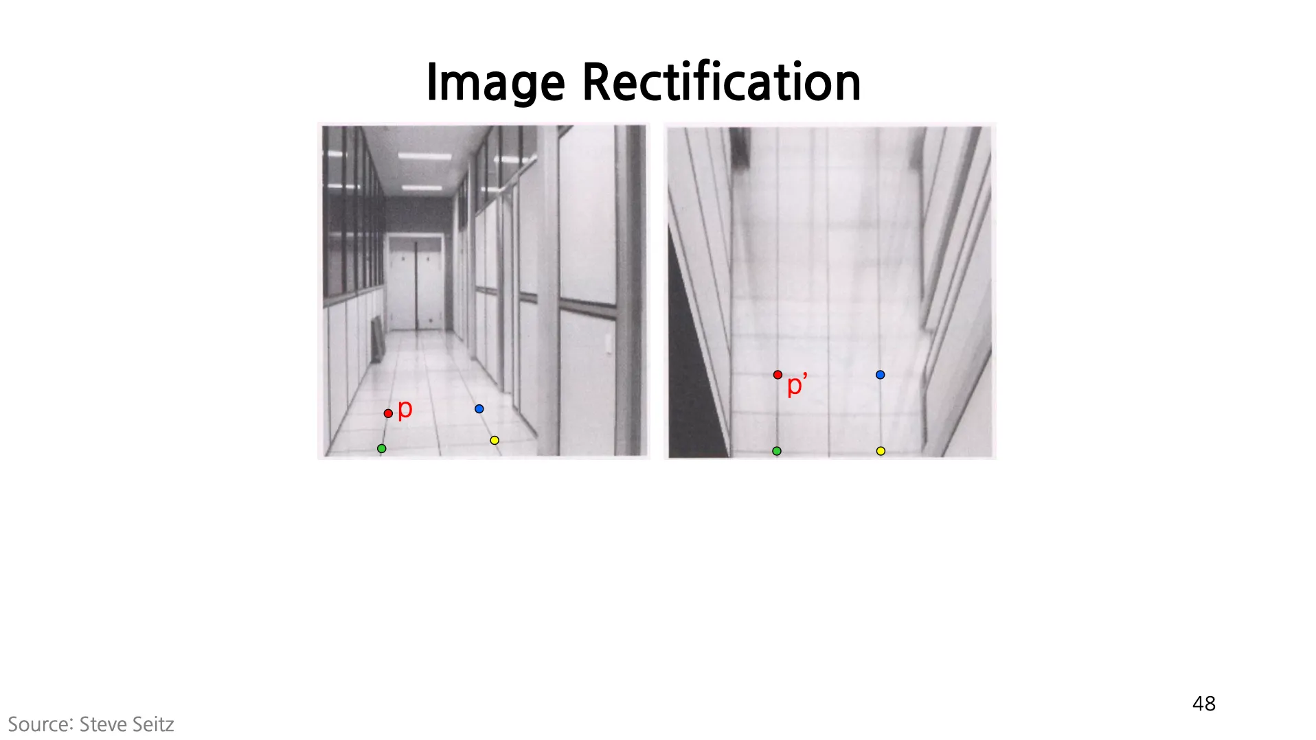
•
원하는 네 개의 지점이 변환된 이미지에서 원하는 네 개의 지점 (위 그림에서는 recangle 형태를 이루도록) 으로 이동하길 원한다- 를 정하면, 이를 통해 transformation (homography) 을 구할 수 있고 변환할 수 있음.
Analyzing Patterns and Shapes + Application
•
이미 알고 있는 (유명한 성당의 바닥 등) 정보를 추가적으로 이용하여 하나의 이미지만으로도 원하는 뷰의 모습을 얻어낼 수도 있음.
•
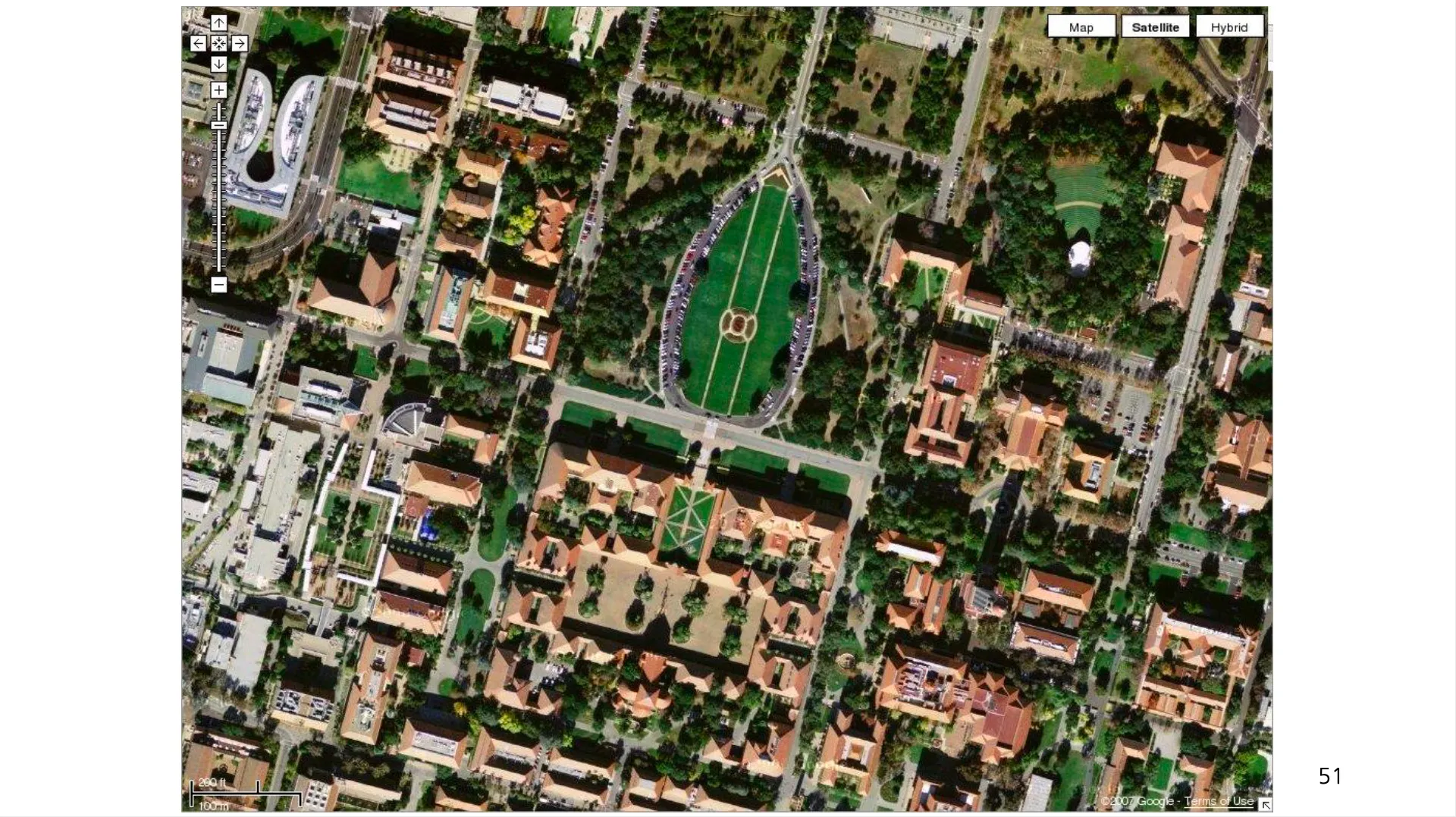
항공사진의 연속적, 불균형한 사진들을 이용해 파노라마를 만들 수 있음.
Summary: Alignment & Warping
•
2D transformations
◦
2D Matrix 형태로 표현할 수 있는 translation 과 같은 transformation 들이 존재
•
Fitting transformations
◦
두 이미지에서 선택한 Corresponding Point Pairs 를 이용해 unkown parameter 를 구하는 과정 (Affine, Homography) 를 다룸
◦
Outlier 를 제거하고 inlier 를 선택하는 RANSAC
•
Perform Image Warping
•
Mosaics
◦
동일한 center of projection 에서 찍힌 여러 장의 이미지를 Homography 와 Image Warping 을 통해서 merge 하는 과정