


2D Projective Transformations
•
실제 세상에서는 직사각형인 것이 이미지 상에서는 그렇게 보이지 않음.
•
실제 세상에서 로 보이는 것이 이미지 상에서는 로 보이는 경우가 종종 있음.
2D Projective Geometry
•
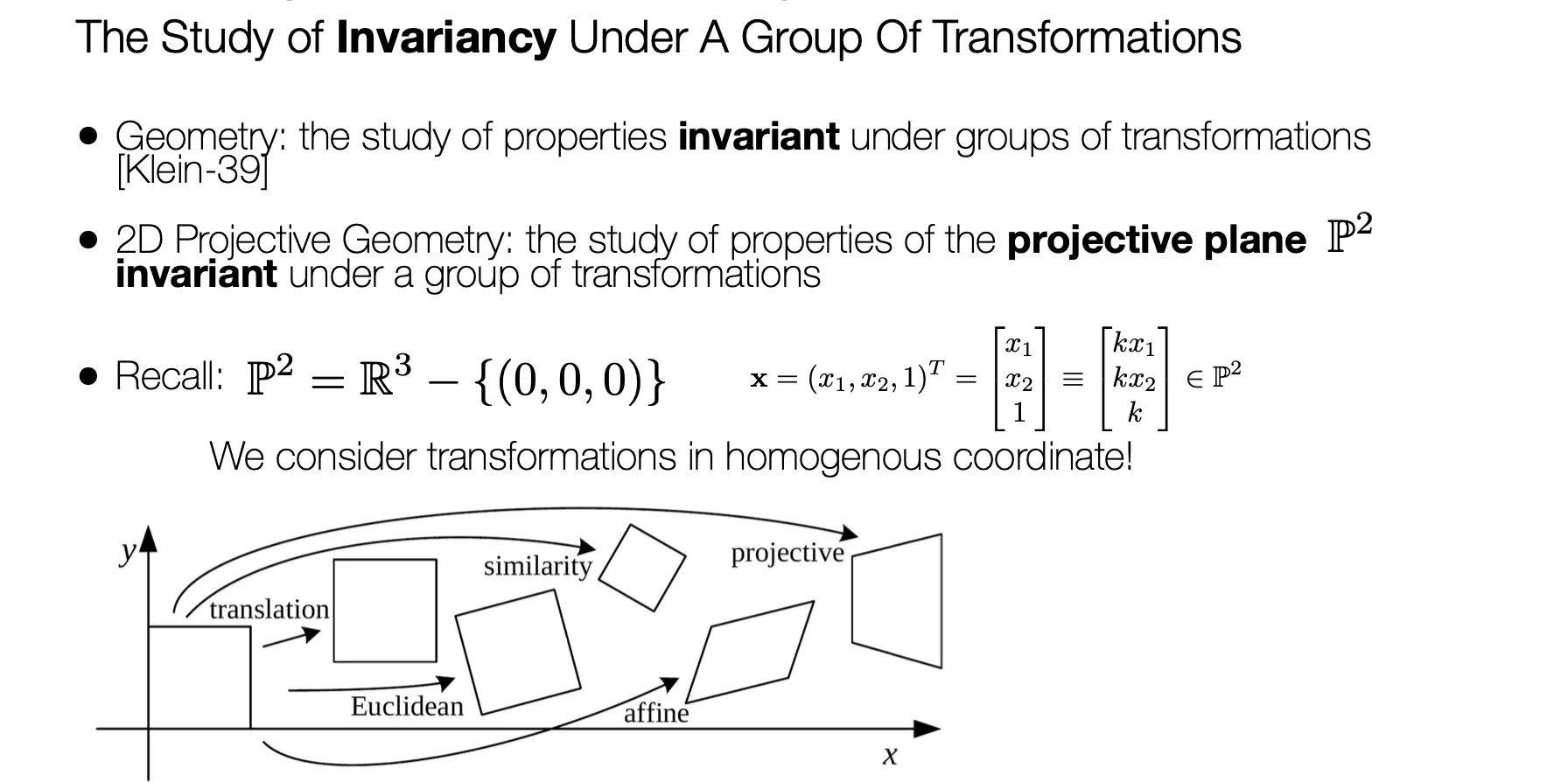
Geometry 는 Transformation 에서 유지되는 invariants 에 대한 연구임.
•
2D Projective Geometry 는 한 Projective Plane 에서 다른 Projective Plane 으로의 변환에서 유지되는 invariants 에 대한 연구임.
Homograph (Projectivity)
•
에서 로의 Invertible Mapping
•
Projectivity == Colineation == Projective Transform == Homography
•
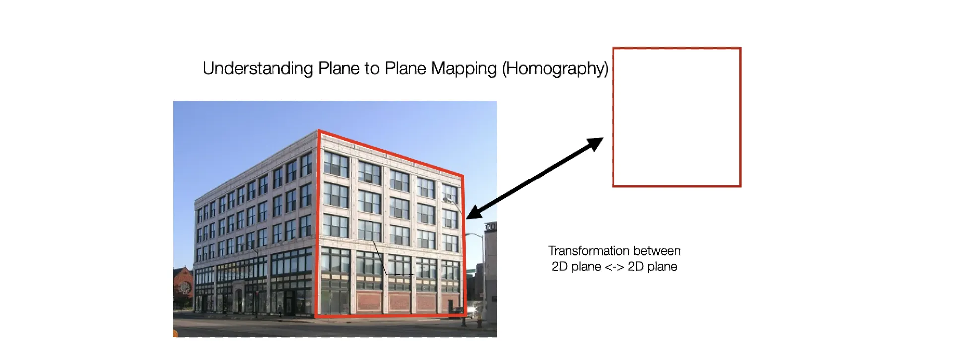
Homography 의 가장 중요한 특성은 Plane-to-Plane Mapping 임.

◦
직선은 다른 Projective Plane 에서도 직선으로 표현됨.
•
Example of Non-Homography Transformation
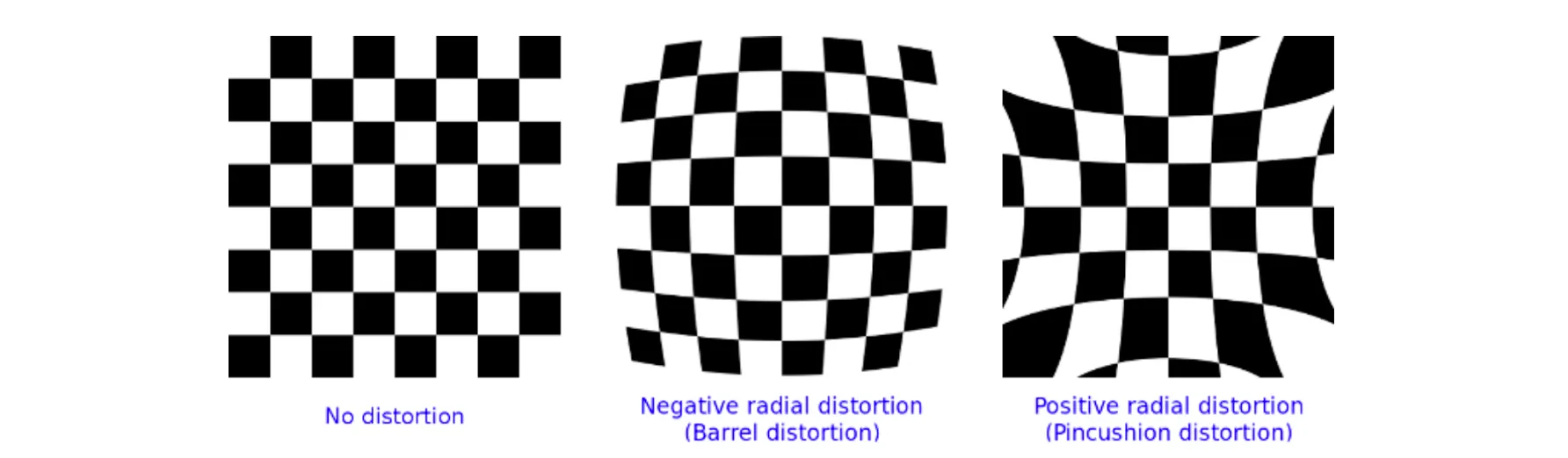
◦
Radial Lens Distorsion 과 같은 현상들이 Non-Homography 임.
Homograph (Projectivity)
•
Non-Singular Matrix 는 모두 Homography 임.
◦
Colinearity 를 보여줌으로써 증명할 수 있음.
▪
밑에서 나오지만 line mapping 은 를 활용함.
•
Homography 는 모두 Non-Singular Matrix 로 표현할 수 있음.
•
Homography 는 Up-to-Scale 임. (좌표 자체가 Homogeneous Coordinate 이므로!)
◦
9DoF - 1DoF (Up-to-Scale) = 8DoF
Homograph (Projectivity)
•
점에 대한 변환이 이면, 동일한 변환은 선에 대해서는 로 표현할 수 있음.
•
증명은 다음과 같음. (Line Form 식이 동일하면 값도 동일하다는 가정 필요)
Homograph (Projectivity)
•
점에 대한 변환이 이면 Conic 에 대한 변환은 로 표현할 수 있음.
•
증명은 다음과 같음. (Conic Form 식이 동일하면 값도 동일하다는 가정 필요)
More Examples using Homography
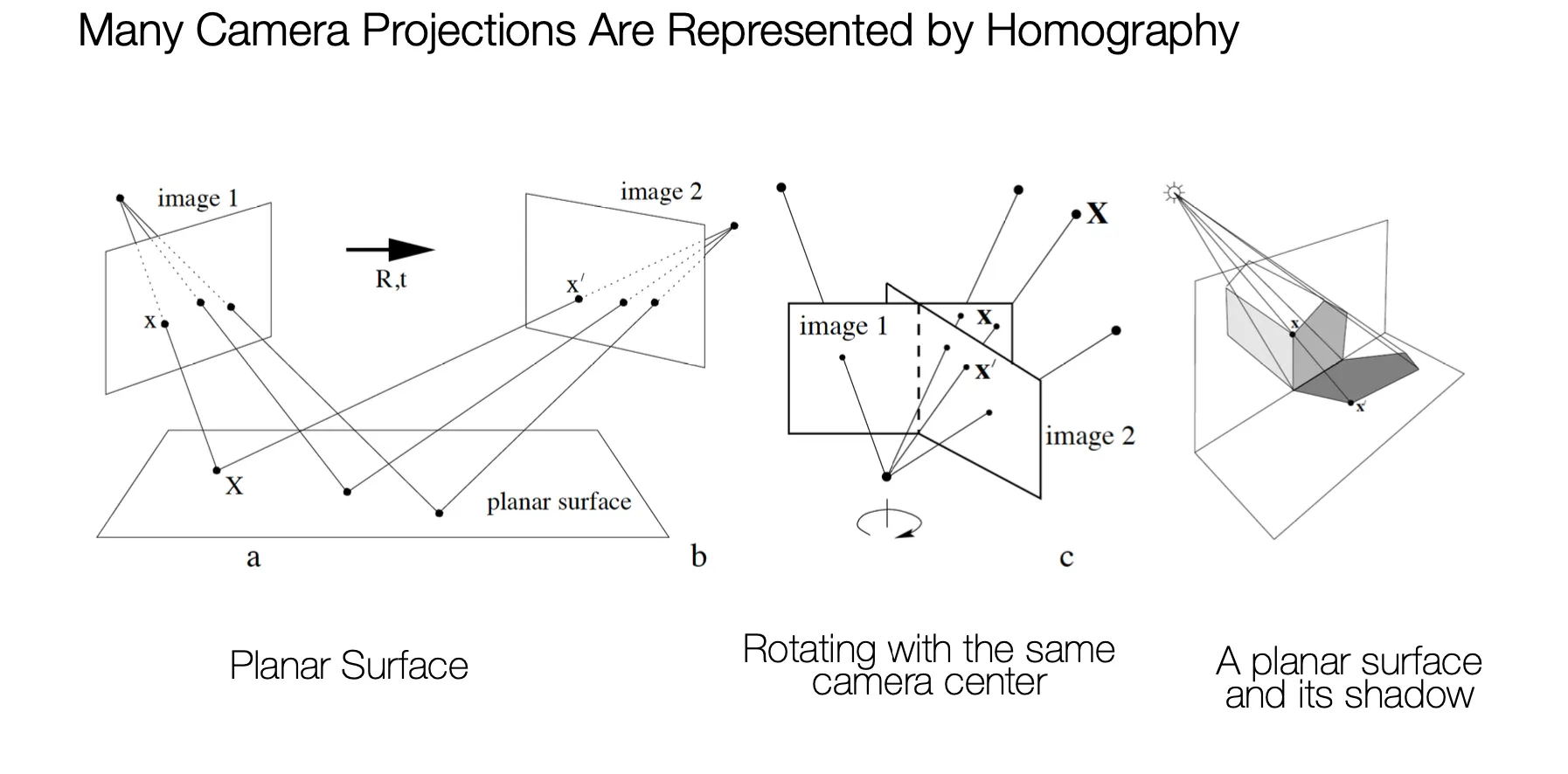
•
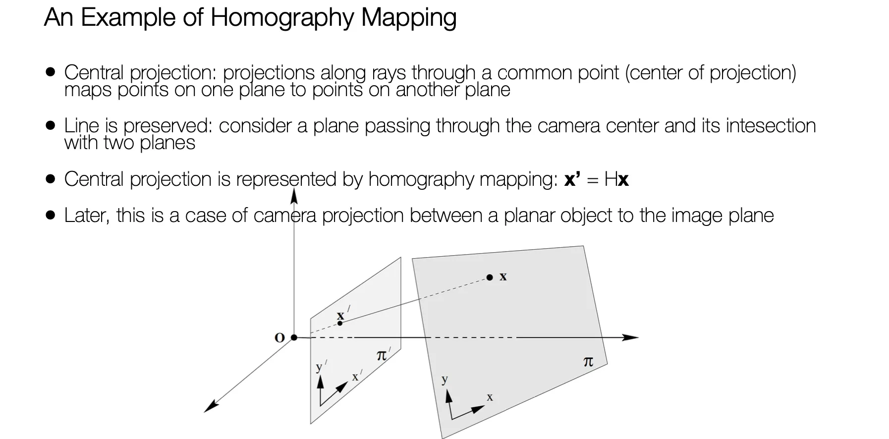
Central Projection
◦
카메라 위치는 고정하고 view direction 과 focal length 만 달리 할 경우도 Homography 로 나타낼 수 있음.
•
Planar Surface
◦
Planar Surface 에 한 번 상이 반사되고 다시 다른 Image Plane 에 맺혔을 때의 결과도 Homography 로 나타낼 수 있음.
•
Rotating Camera
◦
카메라의 위치 및 focal length 를 고정하고 direction 만 회전시킨 경우도 Homography 로 나타낼 수 있음.
•
Planar Surface and Shadow
◦
그림자까지 Homography 로 나타낼 수 있음.
A Hieararchy of Transformations: Transformation
•
좌측: Inhomogeneous Coordinate, 우측: Homogeneous Coordinate
•
Homogeneous Coordinate 은 Matrix Multiplication 이므로 연속적인 변환이나 역변환을 하기에 용이함.
•
2DoF for
A Hieararchy of Transformations: Euclidean Transform (Translation + Rotation)
•
좌측: Inhomogeneous Coordinate, 우측: Homogeneous Coordinate
•
은 다음과 같이 표현됨.
◦
자체는 1DoF (변수는 하나 뿐임)
◦
Rotation Matrix 가 되려면 1. Orthonormal + 2. 의 두 조건을 만족해야 함.
▪
이 두 조건을 만족하는 것들을 Special Orthogonal Group, SO(N) 이라고 부름.
▪
3D Vision 에서 자주 등장하는 Rotation Matrix 는 3DoF 인 임.
•
길이, 각도, 넓이, 순서 (reflection 이 없기 때문에 유지되는 term) 이 유지됨.
•
3DoF: 1DoF for + 2DoF for
•
두 Euclidean Transformation 의 연속적인 변환은 하나의 Euclidean Transformation 으로 나타낼 수 있음. → Matrix Multiplication 해보면 같은 형태가 등장함으로 증명할 수 있음!
Rotation and Translation
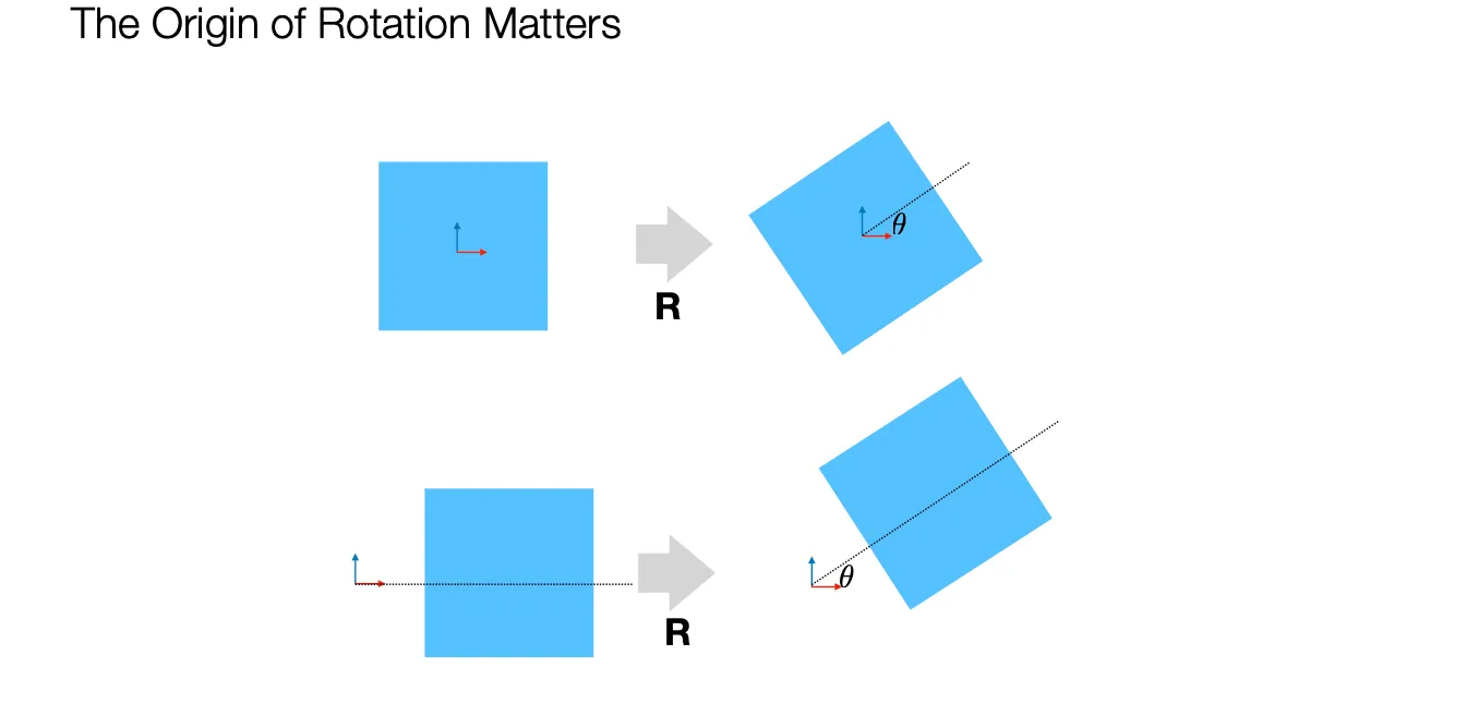
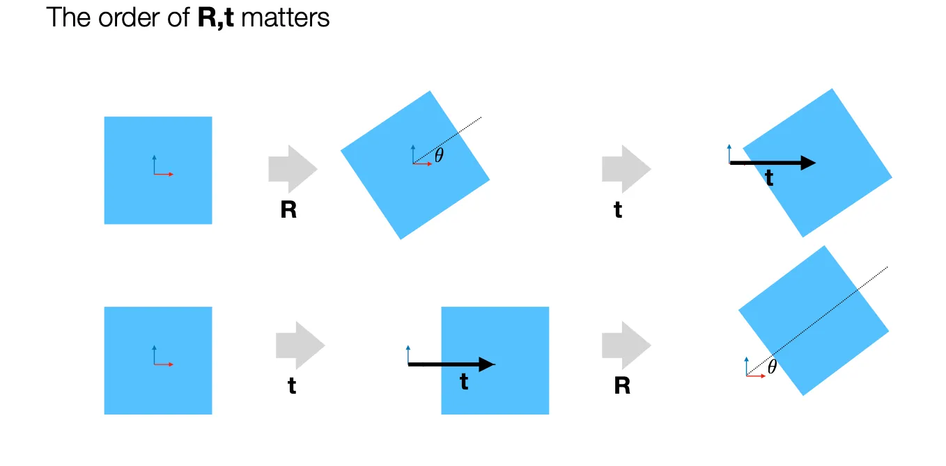
•
Rotation 의 중심에 따라서 결과가 달라짐.
◦
위 결과 때문에 Rotation 과 Translation 의 순서에 따라서 결과가 달라짐.
•
일반적으로 Rotation First, Translation Later 를 따름.
A Hierarchy of Transformations: Isometries
•
Euclidean Transform 에서 term 이 추가된 경우임.
•
•
인 경우는 reflection 이 포함된 transformation 으로 볼 수 있음.
•
길이, 각도, 영역이 유지됨.
A Hierarchy of Transformations: Similarities
•
Euclidean Transform 에서 term 이 추가된 경우임.
•
는 scaling factor 로 확대/축소가 가능함.
•
4DoF: 1DoF for + 2DoF for + 1DoF for
•
각도가 유지됨.
A Hierarchy of Transformations: Affine
•
는 Non-Singular Matrix (Invertible)
•
6DoF: 4 for + 2 for
◦
세 번째 요소를 계산할 때 Up-to-Scale 하지 않음.
•
Parallelism 이 유지됨.
◦
두 평행한 선의 교점 (Ideal Point)을 Affine Transformation 하면 항상 Ideal Point 인 것을 통해 증명할 수 있음. (Invariance of Ideal Point)
◦
Line at Infinity 또한 마찬가지로 Line at Infinity 로 mapping 됨.
▪
Homography Matrix of Point 의 inverse transpose 가 line 끼리의 변환임을 사용함.
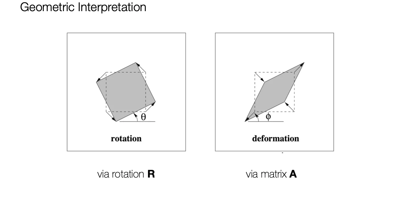
•
는 일반적으로 다음과 같이 표현될 수 있음.
◦
먼저 만큼 회전시킨 뒤에, 특정 방향 () 으로 Scaling 하는 것을 의미함.
◦
다음과 같이 SVD 로 각 항목을 분해할 수 있음.
A Hierarhcy of Transformations: Projective Transformations
•
8DoF: 9 variables - 1DoF for Up-to-Scale
•
는 0 이 될 수 있음.
•
Colinearity, Cross-Ratio 가 유지됨.
A Hierarhcy of Transformations: Summary
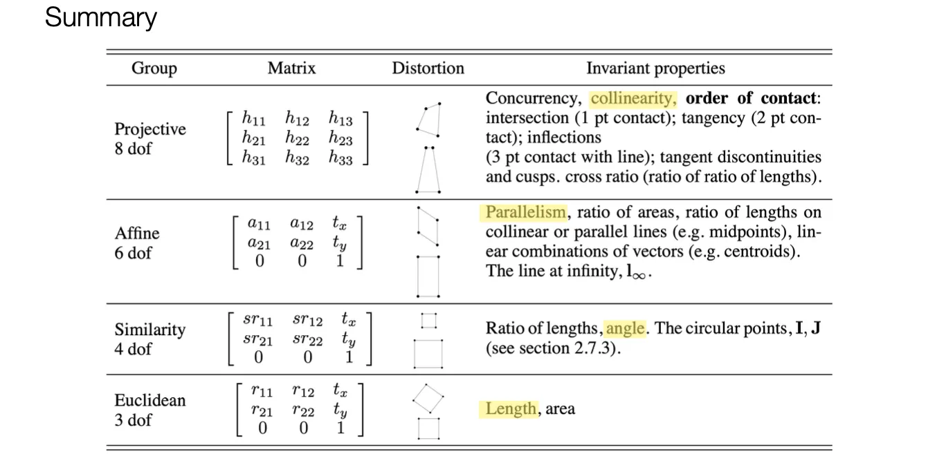
\