Question 1: Epipolar Geometry
Consider two images and that have been captured by a system of two cameras, and suppose the fundamental matrix of two images is known (note that the matrix satisfies the equation for any correspondence two pixel points between images and ). And the epipoles are and . Answer the following questions.
a.
(4 points) Let and , what do and look like? Draw the figures.
Without loss of generality, let’s consider only , and set . For arbitrary points on image plane which is an effective focal length, the equation changes as below.
Since we consider the points on image plane, we can consider as constant and the equation becomes the format of line ().
Therefore, both and look like a green line on image plane as below.
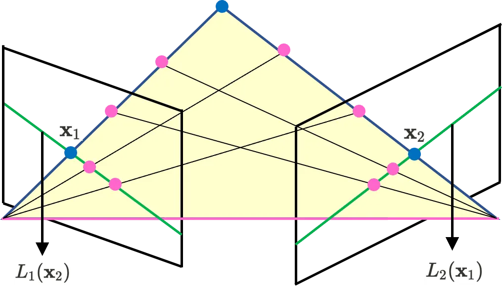
The blue point on left side is on image plane and the blue point on right side is on image plane . The blue point in middle is the exact 3D position which is corresponding to and . The green line on left image plane is and the green line on right image plane is .
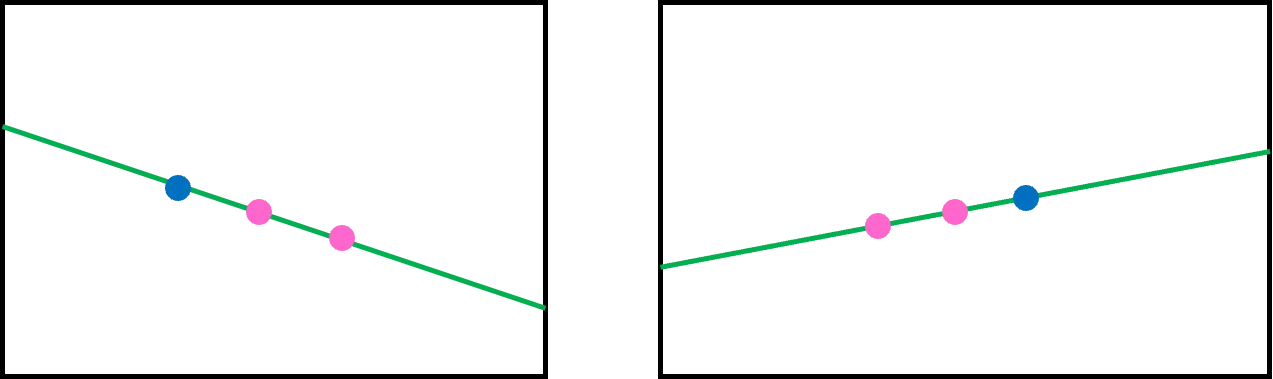
The view on each camera is such as below.
b.
(3 points) Derive .
Remind that every epipolar lines pass through epipole.
For all , is epipolar line on which includes epipole (). Therefore, the below equation is satisfied.
Then, we can apply transpose on each side of the equation to form the equation as below.
Let’s focus on term and assume .
Then for and , should be satsified by equation . Since is expressed as homogeneous coordinate and on image plane , to prevent image plane on infinite. Thus, must be 0. Then there one or more values in must be nonzero by assumption.
Without loss of generality, let’s consider the case of . Then we can consider which sastisfies . Then we can consider , the right side pixel of the (). For , we can calculate the first element of as . This contradicts with equation .
Thus the assumption is wrong and we can safely say that . Since the homogeneous coordinate doesn’t defined on , and this means that has nonzero vector which satisfies , has non-zero nullity which means non-invertible and . Thus we can say since determinant of transpose matrix is same as the determinant of original matrix.
c.
(3 points) In general, is unknown. Explain the 8-points algorithm to obtain with some
correspondence two pixel points
The 8-points algorithm is method for finding unkown fundamental matrix. For one pair of points , we can apply epipolar constarint as below.
If we set , we can simplify the constraint as below.
We can expand the above equation as below.
Finally, we can modify the equation as matrix multiplication of known terms with unknown term as one column vector.
Since the column vector which consisted of the element of has 9 DoF and it is up to scale, we need 8 corresponding point pairs to construct ( is maxtrix, is above column vector consisted of terms) form to find .
As we’ve done in homography, we can solve above problem by setting the objective as below.
We can apply lagrange multiplier to find the minimum as below.
If we differentiate above equation by to find minimum,
we can figure out the minimum value occurs when is an eigenvector of . Then the corresponding value of our objective changes as below.
To minimize above equation, we have to set as minimum value, thus we have to take as an eigenvector of which has minimum corresponding eigenvalue (including zero). By this way we can find out which consisted of the element of fundamental matrix , and we can reconstruct using .
Question 2: Depth Estimation from Stereo
In the lectures, we discussed depth estimation from stereo images. We can estimate the depth from the disparity of the corresponding points on two rectified images. We will explore one of the simple algorithms, window-based corresponding stereo matching by Sum-of-Squared Differences measures (SSD). In this question, there are both theory and programming problems. You should answer the all problems and implement the functions in .
a.
(3 points) Derive the depth of the point, which is defined by the distance from baseline, in terms of , , (where is the distance between two optical centers, is the disparity of two corresponding points, and is the effective focal length).
Let’s consider the system with two cameras which have parallel opical axis as below.
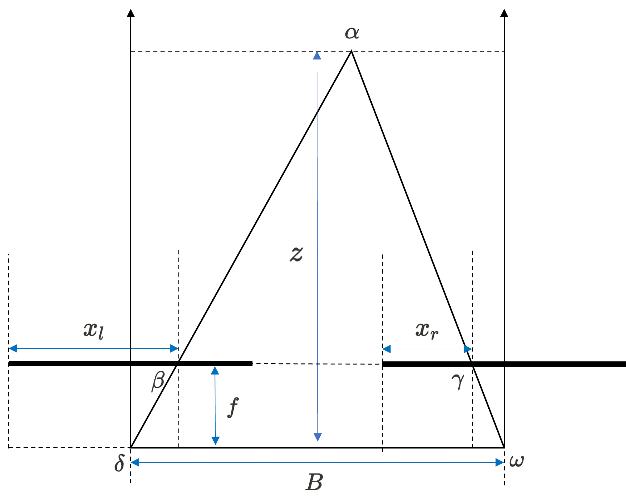
Then, we can find triangle and is similar. Thus, we can say the height bootom line ratio of two triangle is same as below. (let as half width of image plane)
Thus, we can compute depth as below.
Let the rectified images be and , and the window size be (practically set to odd number). The naive SSD matching algorithm is defined by Algorithm 1.
b.
(4 points) The above naive SSD matching algorithm has some problems. Explain
why it is wrong in terms of epipolar geometry, and also explain how to fix it.
According to epipolar geometry, we can find the corresponding points on the epipolar line. Then, we have to calculate SSD for all point patches whose center is on the line and this is time-consuming. To deal with this problem, we can set the set the system’s baseline relatively small enough to ensure the corresponding points on exists quite near to the original pixel on we want to find the pair. By applying this setting, we can assume there exists corresponding points near the original pixel.
c.
(12 points) Now, we’re going to implement your fixed SSD matching algorithm
discussed on (b). Complete following functions, and then apply them to the given
image pair L1.png and R1.png.
And also, display the disparity map using function (already implemented), and save it as . Discuss the results in your writeup.
I firstly implement the function which outputs the sum of the square errors of patch and patch around of image with patch size of .
Then, for implementing the function , I firstly padded two images to safely compute by for top, bottom, left, and right.
Then, I assume that is the image obtained from right-shifted camera compared to the camera which took . Thus, when I iterate over pixels and try to find the corresponding matches on the same horizontal line on , I only focused on left pixels to find the match. Also I used parameter to simplify the problem to only find matches inside the range of difference between original pixel.
While iterating over pixels on , I save the pixel displacement between original focusing pixel (which I iterating over) and the maximum showing pixel on to construct matrix and return it
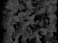
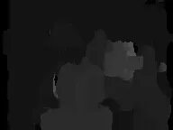
Visualization of image and matrix is as below.
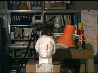
Image L1

disparity_SSD_c(L1, R1)
We can figure out that the bright pixels are nearer (in perspective of direction, depth) than dark pixel which is
d.
(6 points) Apply the algorithm you implemented on to and . and save it as . Also, compare the result and explain why it fails. Can you improve your SSD algorithm to mitigate this issue? Complete the function
Apply this to two pairs and again, and save each of them as 3
and
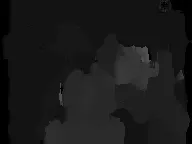
If there isn’t brightness consistancy on two images, I could check the -based implementation failes to estimate depth as below.
disparity_SSD_c(L1, R2)
Thus, I implement new algorithm intuited by normalized cross correlation. Since there might be wrong match when the image scale is different in general matching problem, we could use normalized cross correlation. In this case, I used normalized SSD, which normalize two patch region with L2 norm, and then compute SSD.
disparity_SSD_d(L1, R1)
disparity_SSD_d(L1, R2)
As shown in above images, I could successfully find the depth map using normalized SSD.
Question 3: Motion and Optical Flow (20 points)
a.
(4 points) Give an example of a sequence of images from which you could not recover
either horizontal or vertical components of motion. Explain in terms of number of
knowns and unknowns of the optical flow equation.
Below figure is an example of sequences of images we could not recover horizontal component of motion. (Each number is pixel intensity)

Consider optical flow eqation .
For point , we can figure out , , . Thus, we can construct optical flow equation as below. (We define left, up most pixel is and right, down direction increases each coordinates)
Thus, we can figure out .
However, for other points, we can only construct same optical flow equation as above. Therefore we cannot know about the information of . (For two unknowns and , we cannot figure out one unknown )
b.
(4 points) Give an example of a sequence of images from which you could always
recover horizontal or vertical components of motion. As in , explain with regards
to knowns and unknowns.
Below figure is an example of sequences of images we could always recover vertical component of motion. (Each number is pixel intensity)

Consider optical flow eqation .
For point , we can figure out , , . Then we can construct optical flow equation as below. (We define left, up most pixel is and right, down direction increases each coordinates)
For point , we can figure out , , . Then we can construct optical flow equation as below. (We define left, up most pixel is and right, down direction increases each coordinates)
Thus, we can figure out both and as and . (left & down direction) (For two unknowns and , we can figure out both of them.)
c.
(6 points) Consider a situation where the motion of the camera is in the forward
direction. Does the optical flow equation still hold? Find a simple way to figure
out which scene point the object is moving towards.
While the key assumptions of optical flow equation (brightness consistency & small motion) is holded, the optical flow equation can be still applied on the situation since it is pixel-based method.
However, when camera is moving in the forward direction, the object displayed on image get’s larger and the corresponding region are also expanded. This means that it is hard to easily match the exact region (or pixel) of correspondence. In this situation the brightness consistency cannot be fully applied.
Also, the mapping of 3D point to 2D image plane has the relationship of and if depth becomes smaller (close to the camera), the same amount of the changes makes more and more large amount of changes of and . This means, after the particular timing when object is close enough to camera, the small motion assumption can be not fully applied since occured by small can make large pixel difference.
Thus in general, we cannot say the optical flow equation hold in the situation given.
To figure out which scene point the object is moving towards, we can use depth information and prior knowledge of still objects (such as trees, buildings). By using the still objects (prior knowledge) depth changes in sequence of images, we can compute the camera velocity. Also, we can compute the direction velocity of scene point using depth changes. If the scene point velocity towards camera direction is larger than camera velocity, we can say the scene point is moving towards camera. If it is similar with camera velocity, we can say the scene point is still. (We can also use camera velocity directly if it is given, instead of prior knowledge of still objects.)
d.
(6 points) Consider a camera observing a 3D scene in which each point has the same
translation motion. This means the velocity at each point has the same components.
Show that all the optical flow vectors originate from the same point on the image
plane. This point is called the focus of expansion.
Consider random scene point in time which showing constant translation motion , , . Then we know the corresponding points on image plane is shown as below.
Let’s consider time after situation. Then, the scene point changed to be . We can also know the corresponding points on image plane as below.
Consider the original position of the scene point displayed on image plane. We can compute the position by considering .
The above position is the original rendered position of random 3D scene point having constant translation motion. We can know that the position is unrelated to the specific position of 3D scene point. Thus we can show that all the optical flow vectors originate from the same point on the image plane.
Question 4: Lucas-Kanade Method (45 points)
In this section, you will implement a tracker for estimating dominant affine motion in a sequence of images, and subsequently identify pixels corresponding to moving objects in the scene. You will be using the images in the directory , which consists aerial views of moving objects from a non-stationary camera.
4.1. Dominant Motion Estimation
To estimate dominant motion, the entire image will serve as the template to be tracked in image , is assumed to be approximately an affine warped version of . This approach is reasonable under the assumption that a majority of the pixels correspond to stationary objects in the scene whose depth variation is small relative to their distance from the camera. Using the affine flow equations, you can recover the 6-vector of affine flow parameters. They relate to the equivalent affine transformation matrix as:
relating the homogenous image coordinates of to according to (where ). For the next pair of consecutive images in the sequence, image will serve as the template to be tracked in image , and so on through the rest of the sequence. Note that M will differ between successive image pairs.
Each update of the affine parameter vector, is computed via a least squares method using the pseudo-inverse as described in class. : Image will almost always not be contained fully in the warped version of . Hence the matrix of image derivatives and the temporal derivatives must be computed only on the pixels lying in the region common to and the warped version of to be meaningful.
For better results, Sobel opterators may be used for computing image gradients. So, we have provided a code for them.
a.
(35 points) Lucas-Kanade Method
Complete the following function and explain your code in your writeup:
where indicate and , and is the estimated affine parameter vector.
A naive implementation may not work well. Then, refer to the following tips:
•
This function will probably take too long. Then, try to subsample pixels when you compute the Hessian matrix and . Or, use to calculate the sum-of-product two matrices efficiently.
In this implementation, I totally followed Lucas-Kanadde Algorithm.
First, I normalize my sobel operator result by dividing the gradient values by the sum of the sobel operator elements. This process ensure to keep the pixel scale same as before.
Then, I warp image to match on by applying on warped image’s coordinate and get corresponding pixel value of . To access floating point pixel values in , I use rather than naive bilinear interpolation. By this process, I can get error image.
Then, I have to compute hessian, thus I first compute the term for all position (by using appropriate ) which has dimension of where and is height and width of image . To calculate hessian from this vector, I used matrix multiplication of the previous vector and transpose of it, to get hessian matrix.
Finally, to compute , I have to multiply term with error image elemenwisely (in the term of position) and sum up the result to compute final vector. Then I matrix multiply inverse hessian with the previous vector to finally get and add it to original and return the result.
4.2. Moving Object Detection
Once you are able to compute the transformation matrix relating an image pair and , a naive way of determining pixels lying on moving objects is as follows. Warp the image using so that it is registered to , and subtract it from . The locations where the absolute difference exceeds a threshold can then be regarded as moving objects.
For better results, hysteresis thresholding may be used. So we have provided a code for hysteresis thresholding.
b.
(10 points) Dominant Motion Subtraction
Complete the following function and explain your code in your writeup:
where and indicate and , and is a binary 2D array of the same size that dictates which pixels are considered to be corresponding to moving objects. You should invoke in this function to derive , and produce the aforementioned binary mask accordingly.
To compute the motion image, I have to get appropriate warp defined by which can be computed by previous function . I call the function to get and defined warp function which maps coordinate to .
In the same way I discussed in 4.1, I can get warped image of to match using by using interpolation function . Then, I can safely compute the motion of image by simply subtract the warped image of and .