
Markov Decision Processes
•
Fully observable, Stochastic 한 환경 (Non-deterministic, 확률에 기반)
•
additive reward functions
•
sequential decision problem
•
다음과 같이 구성
◦
Set of states
◦
Set of actions Actions(s) in each state
◦
Transition model
◦
Reward function
•
Policy 는 현재 state 에서 어떤 action 을 택해야 하는지에 대한 함수
•
Optimal Policy 는 highest expected utility 를 가지는 policy
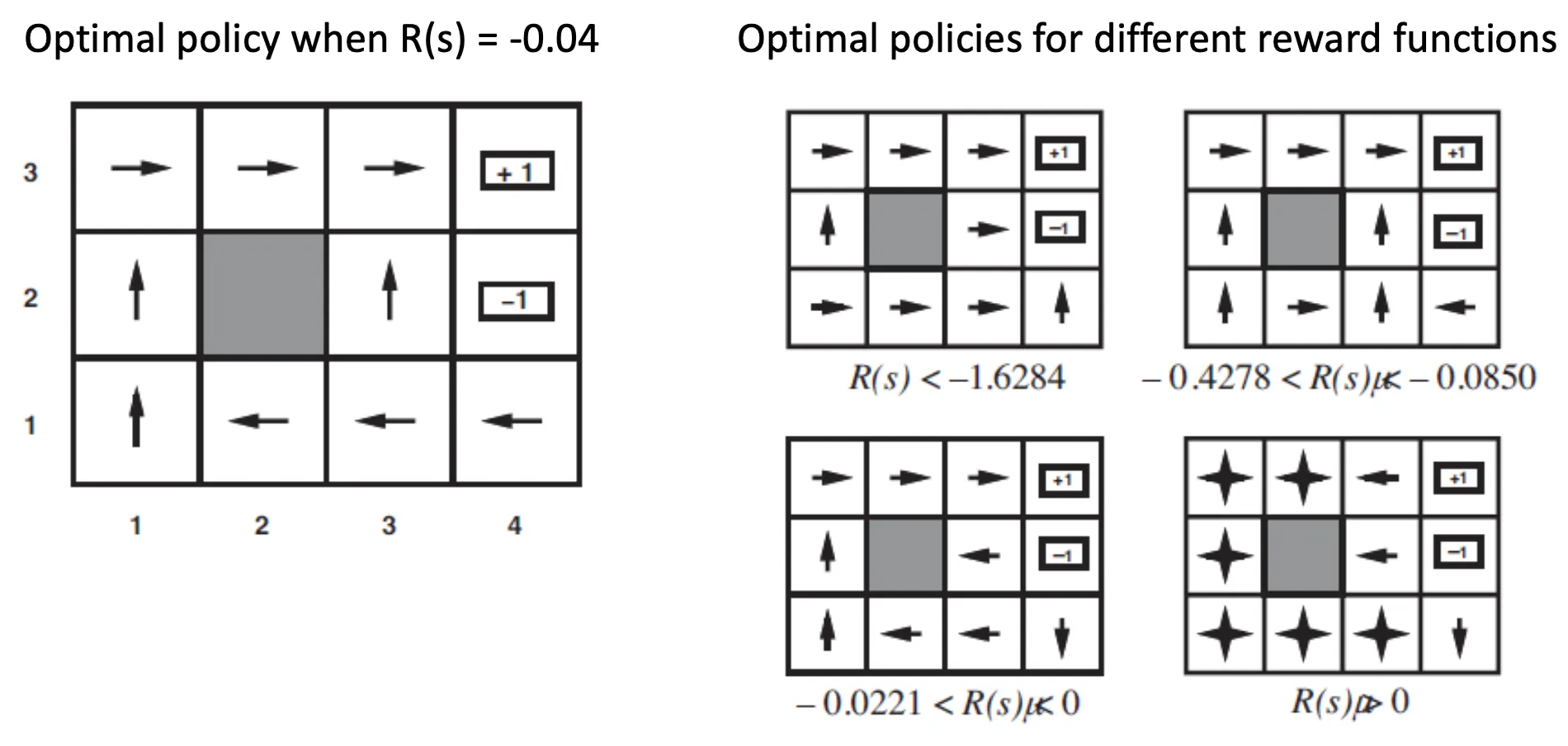
Example of Markov Decision Processes
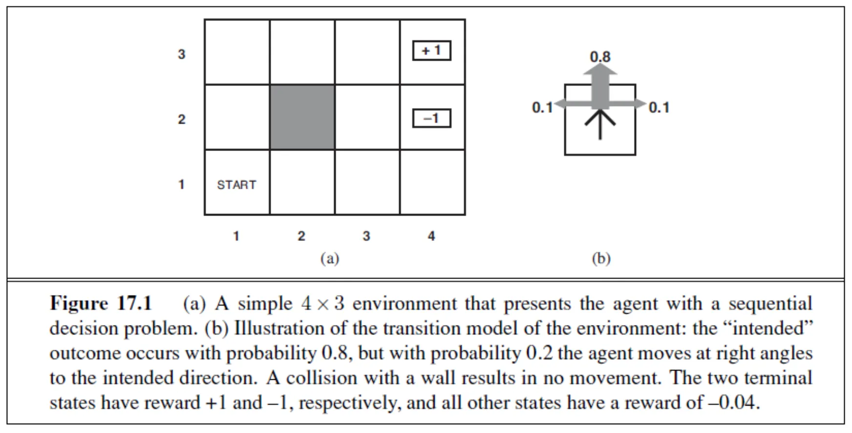
•
각 장소에 부여된 Reward Function 에 따라서 optimal policy 가 달라짐
Utilities Over Time
•
Finite Horizon Problem: 결정 문제가 time 에서 끝남
◦
남은 시간도 condition 개념이라서, 특정 state 에 대한 optimal action 이 time 에 따라 달라짐
•
Infinite Horizon Problem: 결정 문제에 time limit 이 없음
◦
특정 state 에 대한 optimal action 이 time 에 따라 달라지지 않음
◦
Optimal policy 는 시간에 따라서 변하지 않음
Rewards Under Stationarity
•
Additive Rewards
◦
각 state 에서 얻은 reward 의 합이 최종 reward
•
Discounted Rewards
◦
factor 가 지속적으로 곱해진 채로 각 state 에서 얻은 reward 를 합해 최종 reward 결정
◦
로 가정하면, 최종 reward 는 bounded 되어 있음.
Optimal Policy and Utilities
•
Expected Utility by executing starting from
◦
expected utility 를 최대로 만드는 가 optimal policy → 이걸로 만드는 utiliy 가 True Utiliy of State
◦
Infinite Horizon Problem 은 starting state 에 관계 없이 optimal policy 가 동일하다.
•
Principle of Maximum Expected Utility
Value Iteration
•
Bellman Equation
•
n 개의 state 가 있는 경우 n 개의 Bellman Equation 과 n 개의 variable 이 존재
•
Value Iteration 이 optimal solution 을 줄 수 있음
Convergence of Value Iteration
•
Contraction
◦
두 개의 값을 입력으로 받아서 두 개의 출력을 내는데, 출력의 차이가 입력의 차이보다 작아지는 함수
◦
e.g., 2로 나누는 함수
◦
fixed point: function 을 거쳐도 자기 자신인 값 (2로 나누는 함수에 대해서는 0)
•
를 Bellman Update 라고 하고, 이를 utility function 에 적용하다보면, fixed point 인 optimal solution 에 수렴하게 되어 있음. → 복습
•
Discount factor 가 크면 먼 미래를 생각할 필요가 없음.
Convergence Rate
•
Contraction
•
True Utility 에 대해서 ,
◦
때문에 value iteration 은 true utility 로 exponential 하게 converge 함.
•
error bound 미만을 가지기 위해 필요한 iteration 수를 계산할 수 있음. → 복습
◦
Termination Condition
•
Policy Loss:
Policy Iteration
•
Utility Esimate 가 부정확하더라도 optimal policy 를 얻을 수 있음
•
다음 두 단계로 이루어짐
◦
Policy Evaluation
◦
Policy Improvement
POMDP (Partially Observable Markov Decision Process)
•
MDP 와 같지만 state 가 observable 하지 않음
•
Belief State : 모든 state 에 대한 probability distribution
•
observation 에 기반하여 filtering 을 사용하여 를 업데이트할 수 있음
◦
kalman filter 가 한 예시임
•
POMDP 에서 optimal action 은 현재 belief state 에만 기반함
•
Optimal Policy 는 실제 agent 의 state 에 기반하는 것이 아니라 belief state 에 기반함 (agent 의 state 는 관측 불가능하기 때문)
•
state 수가 무한하기 때문에 value iteration 을 적용할 수 없음
From POMDP to MDP
•
Belief-state space 에서 동작하는 transition model
•
Reward function for belief states
◦
reward 에 대한 expectation 느낌
Two Observations
•
physical state 에서 시작하여 고정된 conditional plan 을 실행 시 utility:
•
는 piecewise linear 하고 convex 함 → 두 개의 observation 에 의해 (detail 안 다룸)
Example
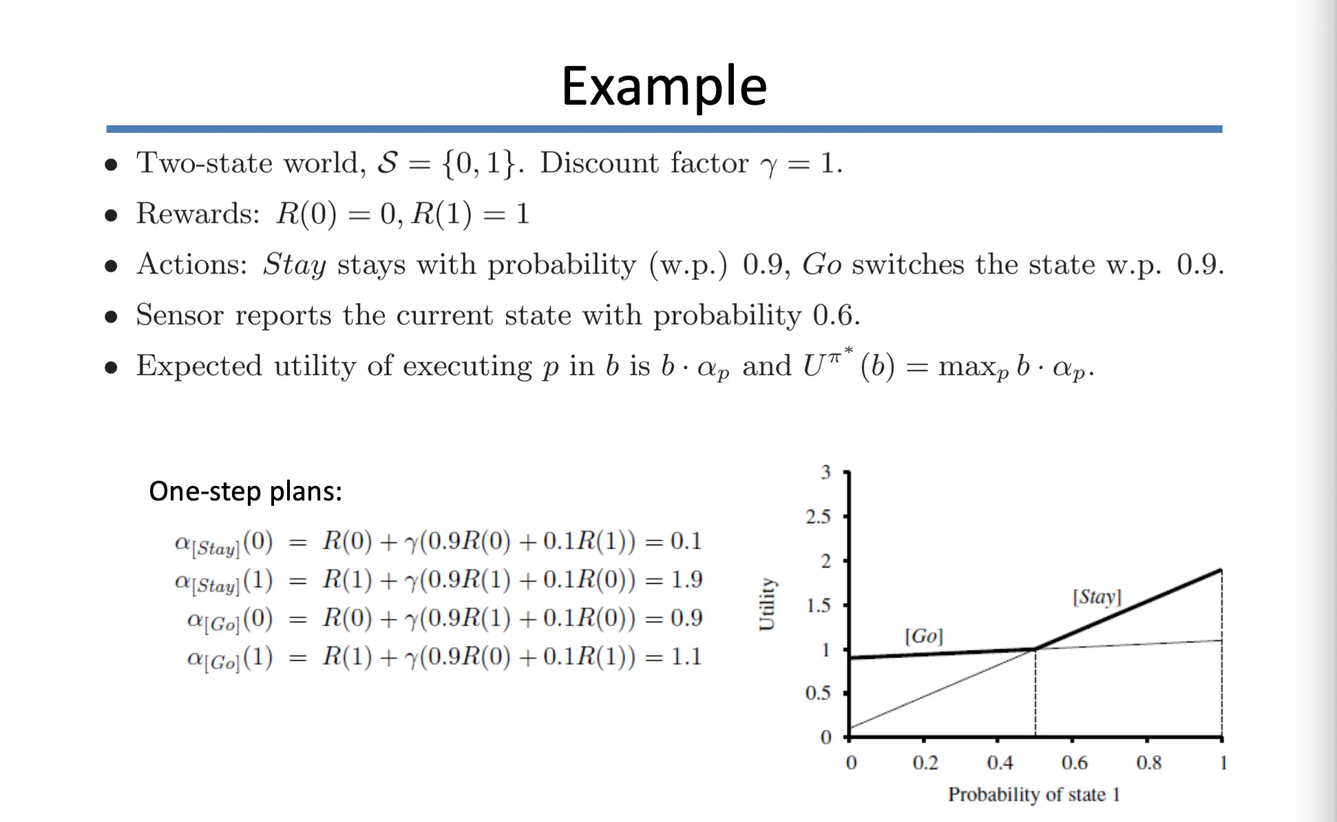
•
위 예시처럼, 를 각각 구할 수 있음
•
probability of state 1 을 vary 함에 따라서 utility 그래프를 그릴 수 있음
Reinforcement Learning
•
MDP 는 complete model 이 알려져 있음 → optimization problem
•
Reinforcement Learning 은 MDP 와 비슷하지만, complete model 이 알려져 있지 않음
◦
Transition Model, Reward 등이 알려지지 않음
◦
관측된 reward (data 를 얻어서) 로 환경에 대한 optimal policy 를 배움
•
세 가지 agent 의 종류
◦
Behavior Cloning: state 에서 action 을 직접적으로 연결하는 policy 를 배움
◦
Utility-based: agent 가 state 에 따른 utility function 을 학습하여 expected outcome 을 최대화하는 action 을 선택함
◦
Q-Learning: → 복습
Passive Reinforcement Learning
Direct Utility Estimation
•
Utility of a state (value of a state or reward-to-go)
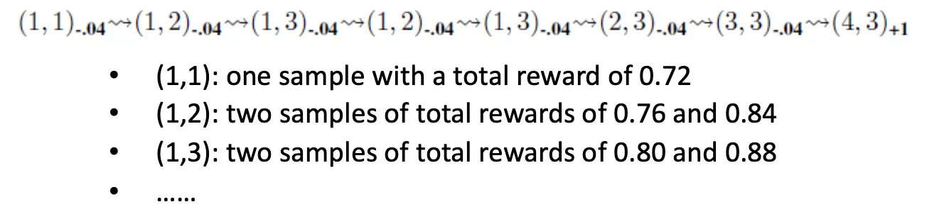
•
Utility function 을 예측하기 위해 supervised learning 을 활용할 수도 있음.
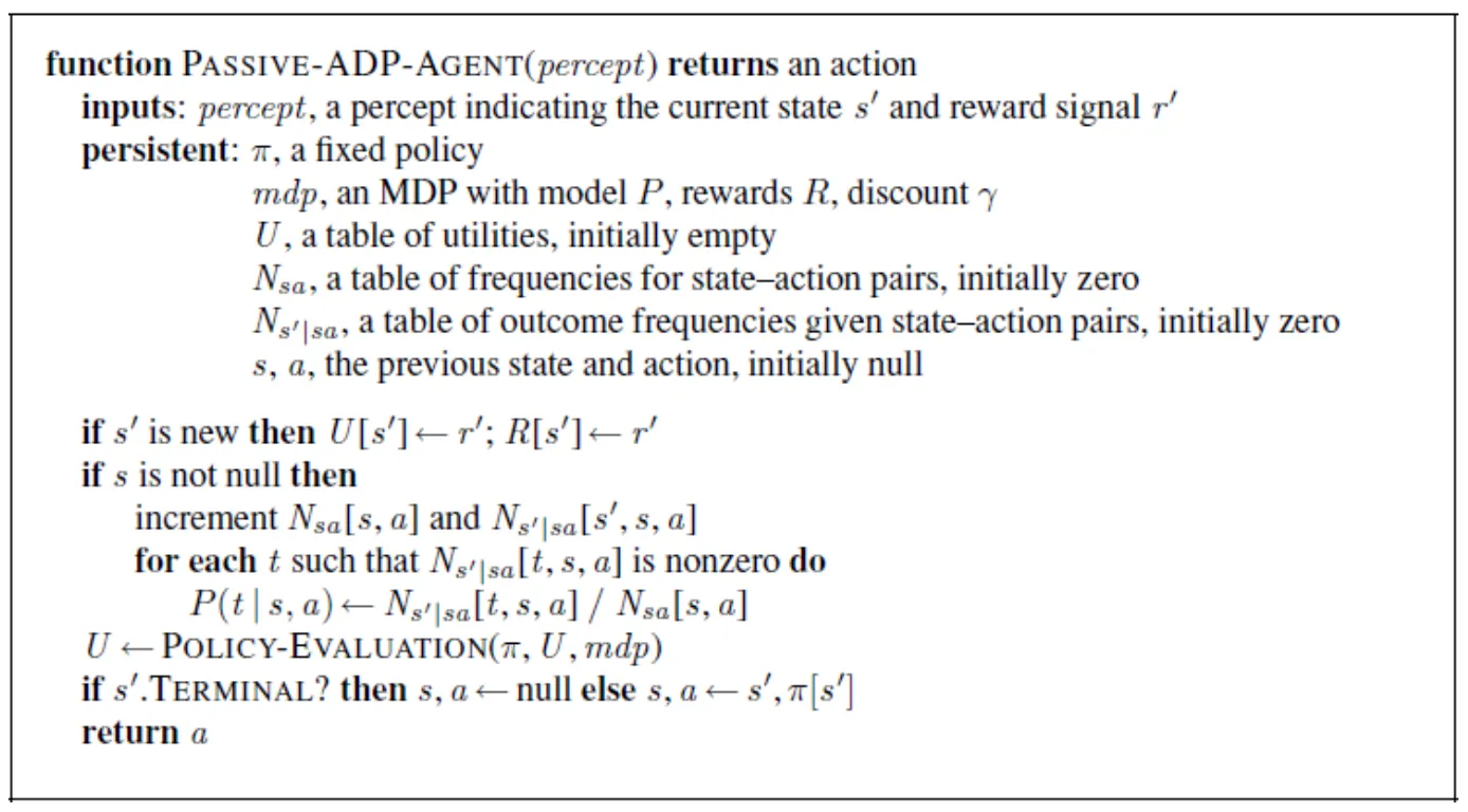
Adaptive Dynamic Programming (ADP)
•
Sample 로부터 transition model 을 배움 (ML estimation)
•
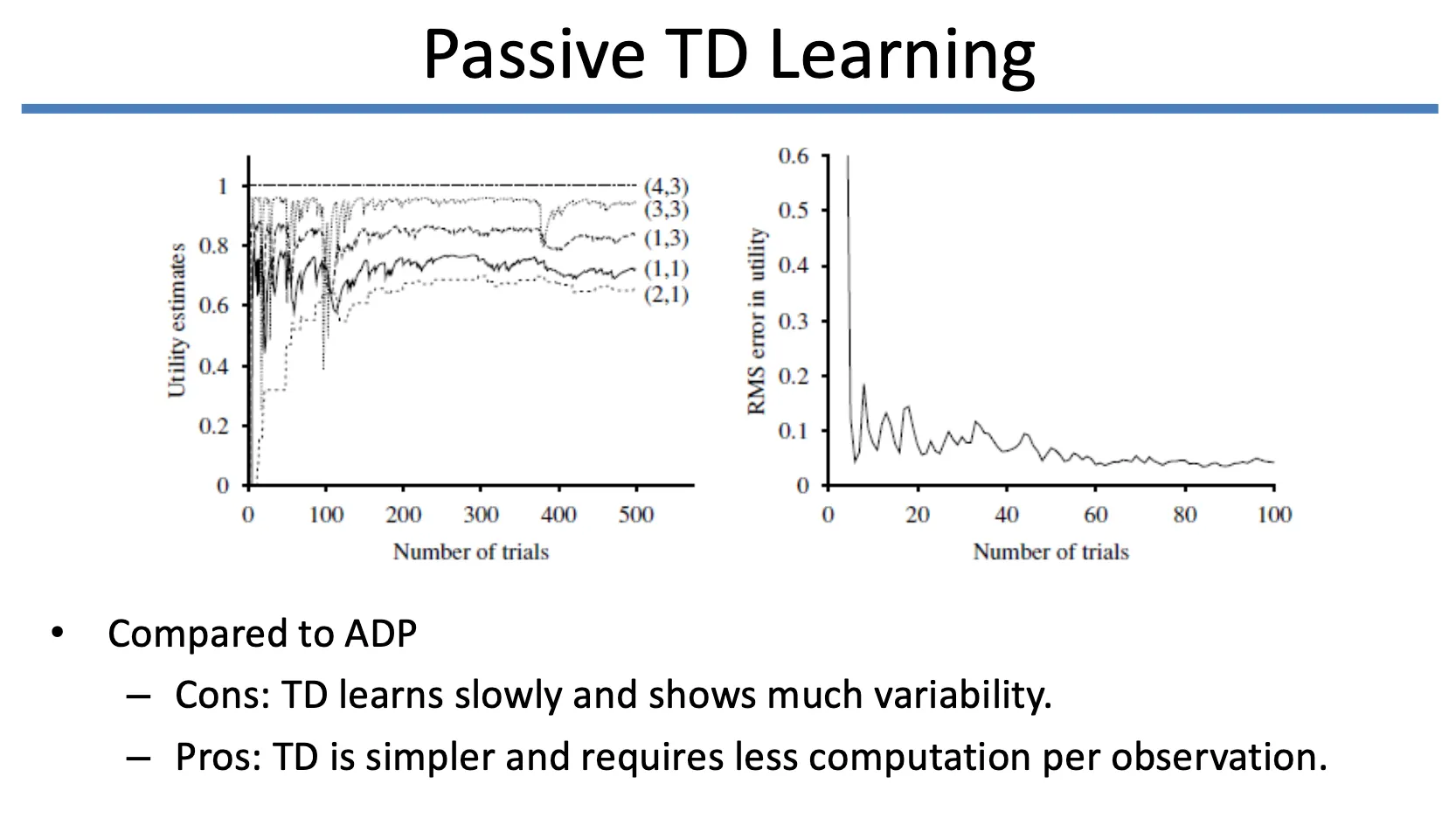
Temporal Difference (TD) Learning
•
Current Estimate 와 One-Step Further Estimate 을 보고
◦
비슷하면, 유지함
◦
one-step 이 크면 현재를 underestimate 하고 있으니 현재 estimate 을 높임
◦
one-step 이 작으면 현재를 overderestimate 하고 있으니 현재 estimate 을 낮춤
•
Gradient descent 와 유사하게 현재의 estimate 을 optimize 함
Active Reinforcement Learning
•
Exploration Function
Action-Utility Function
•
Q function: state 에서 action 를 할 확률
•
Q-Learning 은 model-free 한 방법론임
◦
와 같은, action selection 을 위한 transition model 이 필요없음
Q-Learning
SARSA
•
State-Action-Reward-State-Action
•
Update Rule
◦
maximize function 이 제거된 형태임
◦
greedy agent 에 대해서, SARSA 는 Q-Learning 과 동일함
◦
explorative agent 에 대해서, 다름을 보임
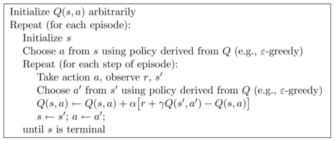
▪
Q-Learning (off-policy), SARSA (on-policy)
Function Approximation
•
Utility function 이나 Q-function 을 유한한 개수의 basis function 으로 근사함.
•
Policy Search
•
Gradient descent 로 policy 를 직접적으로 찾는 방법
•
policy function 을 parameterize (아래 식이 argmax 아니어야 하냐고 언급하심)
•
Policy improvement
◦
Reinforce