


What is the Computer Vision?
•
기계가 사람의 시각을 모방하는 것
•
시각 → Recognition (인지) + Reconstruction (재구성)
Why Vision Important?
•
뇌로 전달되는 정보의 90% 는 시각 정보
•
2022 년에 82% 의 인터넷 트래픽은 온라인 비디오가 차지할 것
•
Robotics, AR/VR, Medical Applications, Autonomous Driving …
Why is Computer Vision Difficult?
•
Ambiguity
•
Variations (Illumination, Object Pose, Clutter, Occlusions, Intra-class appearance, viewpoint)
•
Scale
•
Occlusion
•
Context and Human Experience → Context 나 인간의 경험만으로 완벽하지 못한 판단이 나올 수 있음
A Brief History of Computer Vision
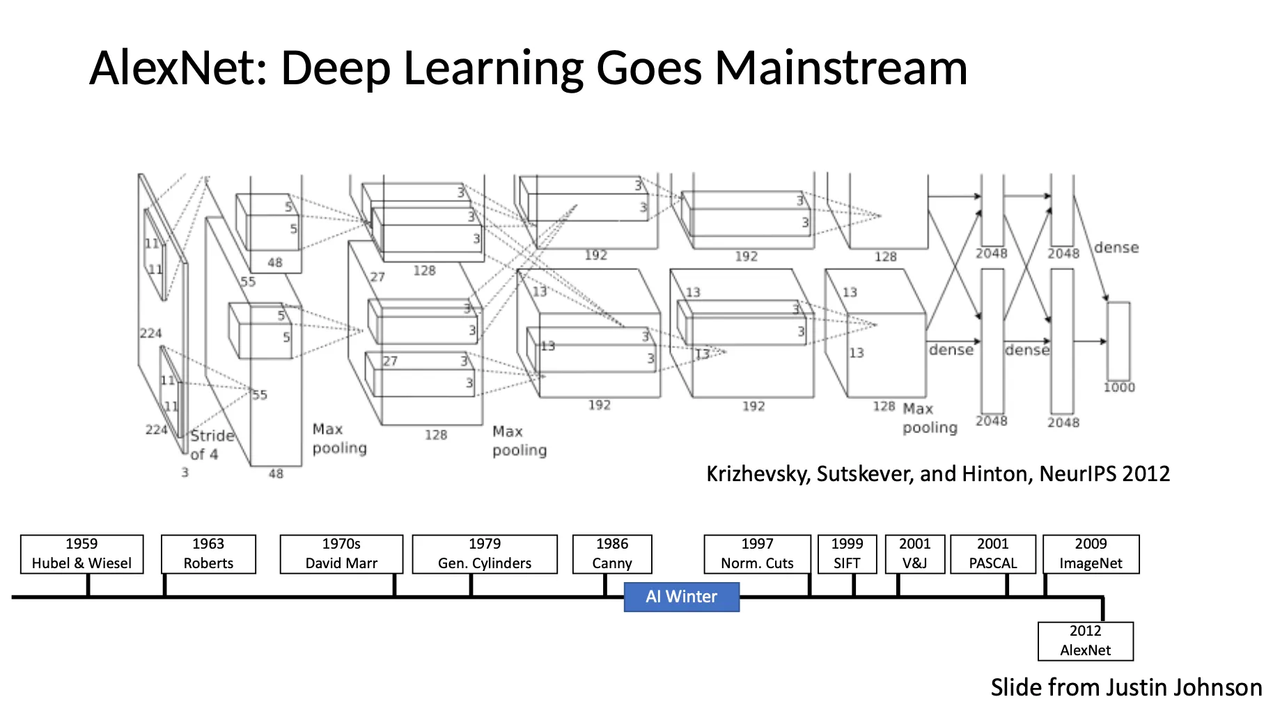
•
Roberts (The Summer Vision Project) → David Marr (Stages of Visual Represenatation) → Recognition via Parts (1970s) → Recognition via Edge Detection (1980s) → Recognition via Grouping (1990s) → Recognition via Matching (2000s) → Face Detection → PASCAL Visual Object Challenge → ImageNet → AlexNet (Deep Learning)
What is the AI we are Talking Nowadays?
•
Traditional Programming 은 if-else 문으로 프로그램을 작성
•
Machine Learning based 방법론은 input 과 output 으로 프로그램 를 만들어냄
◦
Training data 를 잘 설명하는 를 찾아냄
•
는 과거에는 simpler models (ex. linear) 를 사용했지만, 최근에는 neural network 를 사용
◦
Large-Scale data 와 optimization 으로 최선의 parameter 를 찾아냄
◦
알고리즘보다 데이터가 더 중요해졌음!
◦
Hand-design feature 를 뽑아낸 후에 사용할 수도, end-to-end 로 사용할 수도 있음
How To Represent an Image
•
RGB, 3 개의 채널 각각에 까지의 값을 할당
•
Image Filtering
•
Pixel-wise Filtering
◦
→ Brighten
◦
→ Darken
◦
→ Inversion
◦
→ Custom
•
Spatial Filtering
◦
픽셀 하나뿐만 아니라 각 픽셀의 주변을 같이 보면 더 흥미로운 feature 들을 뽑을 수 있음!
▪
: Image to filter over
▪
: Filter
▪
: Filtered image
◦
→ Identity filter
◦
→ Shifting right side 1 pixel
◦
→ Moving average filter
◦
→ Directional blur (Horizontal blurring)
◦
→ Direction blur (Vertical blurring)
◦
→ Gaussian blur
▪
가 클수록 주변 픽셀의 영향이 커지면서 blurring 이 심해짐
◦
가운데가 +, 주변이 - 인 filter → Image sharpening
◦
→ Image differentiation ( direction)
▪
Noise 에 굉장히 민감한 filter 이기 때문에 이를 이용해서 edge detection 을 할 경우 edge 가 아닌 부분도 edge 로 볼 수 있음!
◦
→ Image diffentiation ( direction, sobel filter)
▪
Gaussian + Differentiation 이 합쳐진 filter 로, noise sensitivity 가 낮음!
How to Handle Pixels at Boundary
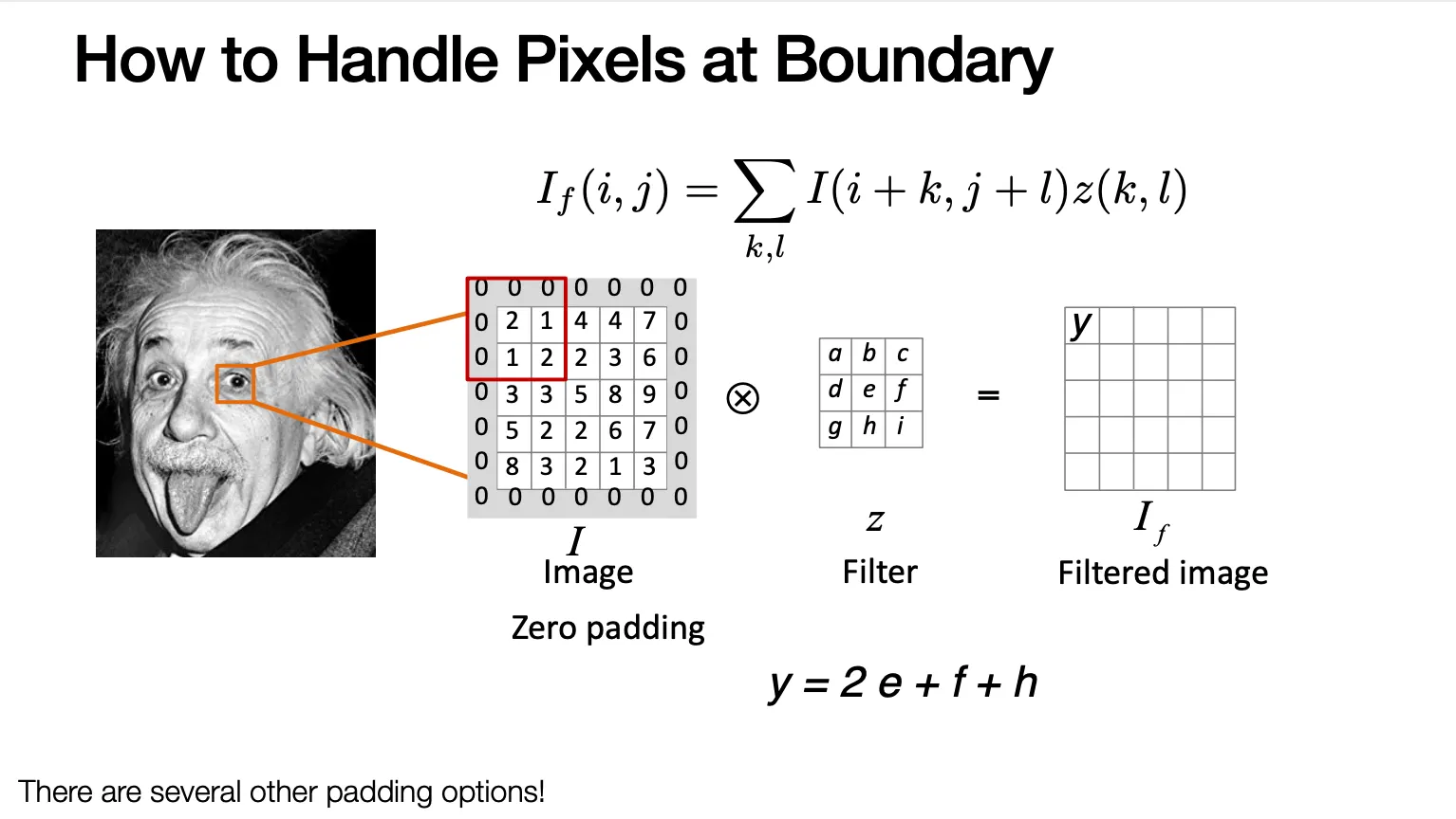
•
이미지 바깥쪽에 0 을 두르는 zero-padding 을 하여 주변값을 채워넣음!
Correlation vs. Convolution
•
Image Correlation
•
Image Convolution
◦
Filter 를 vertical, horizontal 하게 flip 하고 곱해서 더한다는 점이 Correlation 과 다름!
Properties of Convolutions
•
Shift Invariance: 이미지 내부의 위치에 상관없이 filter 내부의 값에만 영향을 받음
•
Commutative:
•
Associative:
•
Superposition, Distributes over Addition:
•
Scalars factor out:
•
Identity: where (unit impulse)
•
Associativity 때문에 linear filter 들을 하나씩 계속 겹쳐 넣은 것이 merge filter 를 넣은 것과 같게 되는 이점이 있음
Convolution as a Feature Extraction
•
사용하는 filter 에 따라서 response 가 달라지고, 이러한 response 를 feature 로 사용할 수 있음!
•
Filter Bank 는 scale, orientation, type 에 따라서 여러 filter 를 모아둔 것으로 다양한 feature 를 뽑을 수 있음
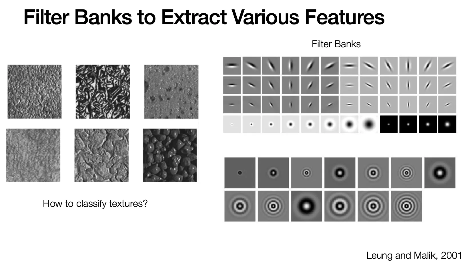
•
Convolutional Neural Network 에서는 optimal 한 filter 가 loss 를 최소화하는 방향으로 data 로부터 자동으로 최적화됨!
Image Gradient
•
Gradient 는 derivative 의 multivariate generalization
•
Magnitude of gradient 는 contrast change (intensity, brightness change) 에 비례
•
Direction of gradient 는 contrast change 가 가장 가파르게 일어나는 방향
Edge Detection
•
이미지에서 edge 는 무엇인가?
◦
Depth discontinuity
◦
Illumination discontinuity
◦
Surface color discontinuity
•
가장 간단한 방법은 magnitude of gradient 를 thresholding 하는 것
◦
이러한 방법은 대게 non-locality (너무 굵은 edge 가 나오는 현상), discontinuity (edge 가 끊기는 현상) 가 나타남
Edge Localization: Non-maximum Suppresion
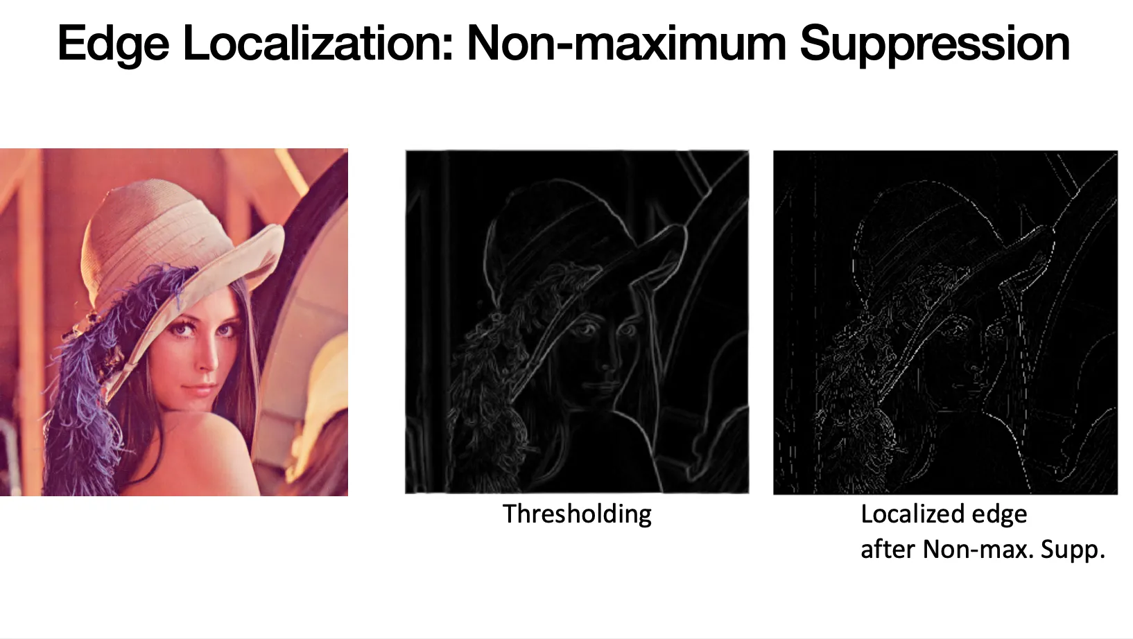
•
Non-locality 의 해결방안
•
Threshold 를 넘어 edge 로 선언된 각 픽셀별로, 해당 픽셀이 가진 gradient direction 의 양쪽 방향으로 이동하여 찾은 두 개의 neighbor pixel 과 gradient magnitude 를 비교하여 본인이 가장 높은 값을 가지지 않으면 해당 픽셀은 edge 에서 박탈함
Edge Linking
•
Discontinuity 의 해결방안
•
Weak edge 로 선언된 픽셀에서 tangent direction 으로 이동하여 발견한 픽셀이 weak edge 면 한 번 더 반복하고, strong edge 이면 해당 edge 와 연결, 그 둘이 아니면 reject 함.
Edge Prediction: Hysteresis
•
두 개의 threshold 를 두어 high threshold 보다 큰 픽셀은 바로 strong edge 로, low threshold 보다 작은 픽셀은 바로 reject 함
•
두 threshold 사이의 픽셀들은 weak edge 로 선언하고 strong edge 와 연결된 픽셀들만 최종 edge 로 선택함
Is Edge Detector Solved?
•
Canny edge detector 가 좋은 성능을 보이고 있지만, 많은 경우에 semantic 한 물체에 기반한 edge 를 그려내지는 못함 → 이 분야의 연구들이 이루어지고 있음
•
ex. Semantic Edge Detection with Diverse Deep Supervision