
Image Intensity and 3D Geometry
•
2차원의 이미지를 보고도 대상 물체의 3차원 정보를 어느정도 예상할 수 있음.
◦
Shadow 정보에 의해서 3차원 정보를 유추할 수 있음.
◦
이미지 픽셀의 intensity 값으로부터 shape 을 유추할 수 있음. → Reflectance Map
Surface Normal
•
3차원 평면:
◦
으로도 표현할 수 있음.
◦
Surface Normal 은 같이 표현할 수 있음.
▪
▪
▪
Gradient Space
•
Normal Vector
•
Source Vector (광원)
•
평면은 Gradient Space 라고 불림.
◦
어떤 orientation 이 주어지던간에 Gradient Space 의 point 로 mapping 이 가능함.
◦
는 source vector 와 normal vector 사이의 각도
Reflectance Map
•
Image Intensity 를 surface orientation 와 관계짓는 것.
•
Lambertian Case (Diffusion Reflection 만 고려)
◦
: source brightness ()
◦
: surface albedo
◦
: normalization constant
◦
Image Intensity
▪
특점 점에서의 Radiance 와 Image Intensity 는 라는 비례상수를 가지는 비례관계
(
▪
로 두면, 가 됨.
▪
Reflection Map 는 다음과 같이 표현됨.
•
Source Vector 와 동일한 각도를 이루는 normal vector 들을 가지는 Surface (Cone 영역의 normal vector 들) 에 대해서는 동일한 Image Intensity 를 가짐. 이러한 normal vector 들은 Gradient Space 로 mapping 하게 되면 타원형태가 됨. → Iso-brightness contour 라고 함.
◦
Gradient Space 상의 Iso-brightness contour 는 아래와 같음.
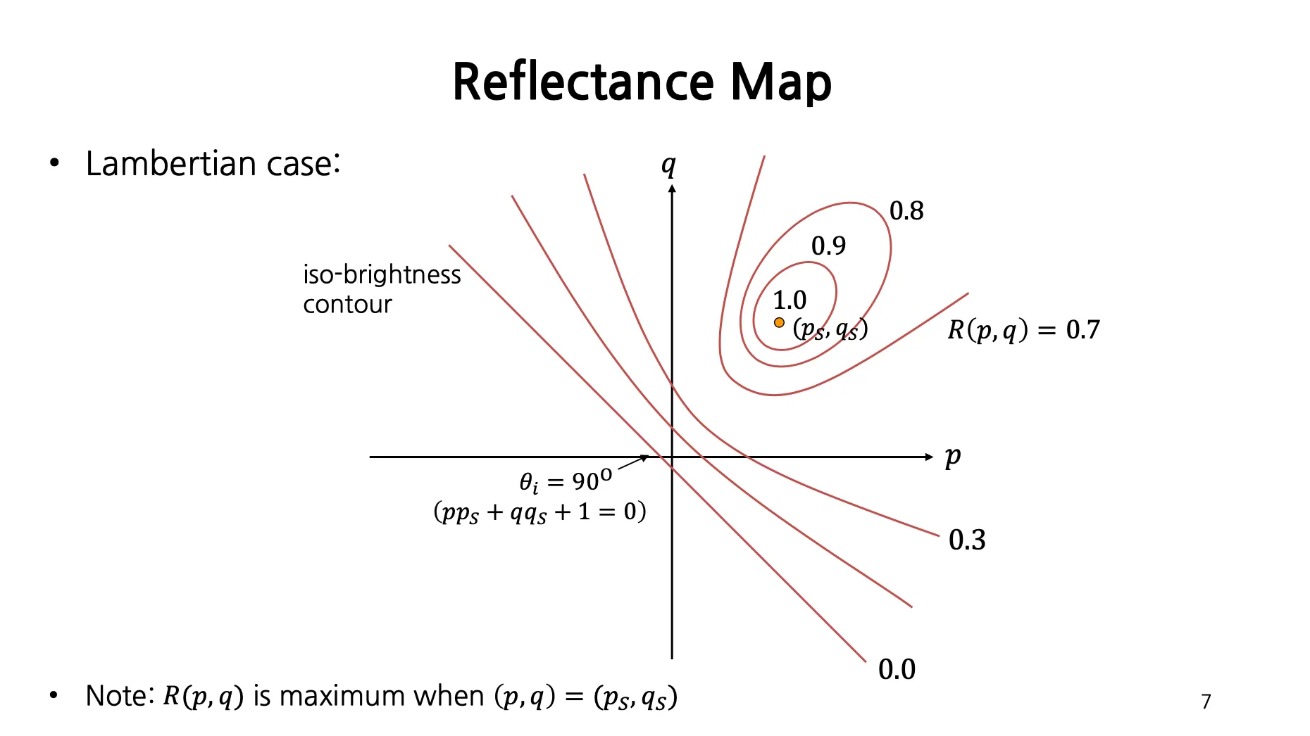
▪
각도가 일 때 값은 1.0 이 되며 점 형태로 그려지고, 각도가 커질수록 값이 작아지며 타원이 커지는 것을 볼 수 있음.
Shape from a Single Image?
•
Source Direction , Sufrace Reflection , Image Intensity 를 알고 있다고 하더라도, surface orientation 를 unique 하게 결정할 수는 없음. (contour 상에 존재하는 여러 점들이 후보가 됨.)
•
즉, 한 장의 이미지만 얻어서는 unique 하게 Surface Normal 을 얻어낼 수 없음.
◦
첫 번째 option 은 사진을 여러 장 찍는 방법임. → Photometric Stereo
▪
물체 및 카메라는 고정한 채로, 광원을 돌려가면서 변화하는 Image Intensity 를 얻어냄.
◦
두 번째 option 은 constraint 를 주어 후보 중 하나를 선택하는 방법임. → Shape-from-Shading (그림자로부터 3D Shape 을 예측하는 방법으로, 강의에서 다루지는 않음.)
Photometric Stereo
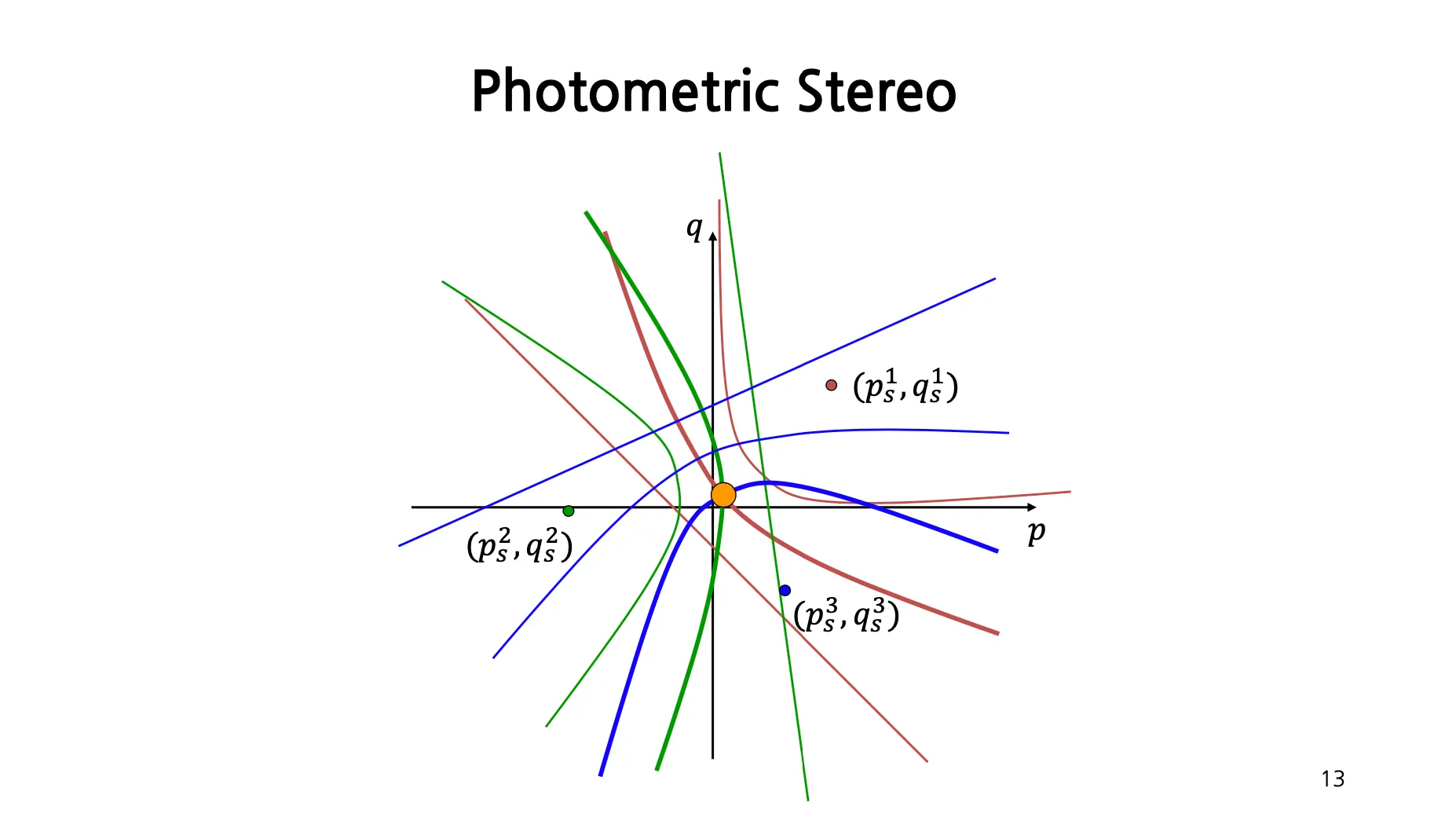
•
광원 , , 에 대해서 Image Intensity 를 추출하고 특정 픽셀이 가질 수 있는 Surface Normal 에 대한 iso-brightness contour 를 그릴 수 있음.
•
Iso-brightness contour 의 교점에 해당하는 가 실제 물체의 Surface Normal 값임.
•
◦
◦
◦
◦
More then Three Light Sources
•
Source Direction 의 측정 오차나 가정등으로 인해서 일반적으로 세 번보다는 많은 광원 위치변경을 사용함.
◦
Ideal 하게는 같아야 하지만, 오차에 의해서 그럴 수 없을 수 있으니 좌변과 우변의 차이를 최소화하는 방법을 사용. (Least Square Solution)
◦
◦
◦
→ Moore-Penrose pseudo inverse
Color Images
•
각 color channel 마다의 equation 을 얻어낼 수 있음.
◦
하나의 equation 만 집중하여 을 얻어낸 뒤에 값들을 대입하여 얻어낼 수 있음.
◦
또는, 세 channel 의 intensity 를 합쳐서 최종적으로 하나의 을 구해낼 수도 있음.
Computing Light Source Directions
•
앞서 Surface Normal 을 구하는 Photometric Stereo 방법론은 Light Source 의 direction 이 주어져야 진행할 수 있었음.
•
직접 Light Source 를 컨트롤할 수 있다면 문제가 없지만 그렇지 못한 경우에 접근할 수 있는 방법론을 생각해볼 필요가 있음.
Specular Reflection - Recap
•
정확히 반대 방향으로 모든 빛이 반사되는 경우가 Specular Reflection.
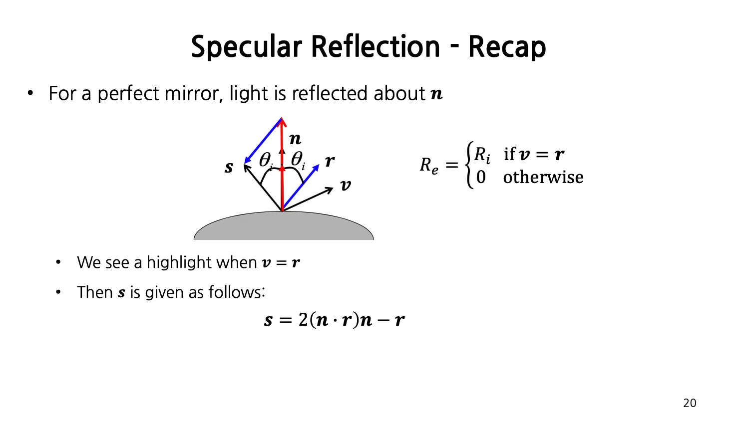
•
구체의 highlighted 된 위치는 view direction 과 반사되어 나가는 빛의 direction 이 같아질 때 () 나타남.
◦
과 을 알고 있으면 source direction 를 구할 수 있음.
•
은 카메라의 방향과 같을 때 highlighted region 을 생각하는 것이므로 구할 수 있음.
•
의 경우에는 아래와 같이 구할 수 있음.
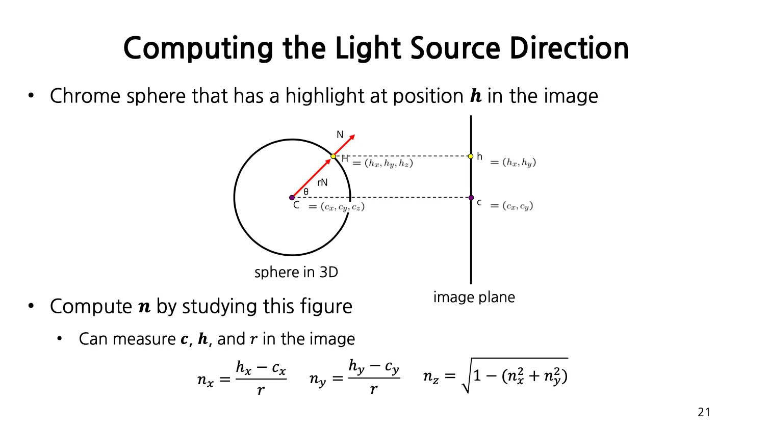
◦
, 는 이미지 상에서 highlighted 된 부분의 좌표
◦
, 는 이미지 상에서 구체의 중심 좌표
◦
은 구체의 반지름
◦
, ,
Limitations
•
Big Problems
◦
Lambertian Surface 는 이상적인 Surface 이기 때문에 반짝이거나 반투명하면 잘 동작하지 않음.
◦
Shadow 에 해당하는 부분은 Surface Normal 을 알아내기 어려움.
◦
완전이 control 된 방이면 좋은데 inter-reflection 이 심한 곳 같으면 동작하기 어려움.
•
Smaller Problems
◦
카메라와 광원이 충분한 거리를 두고 떨어져 있어야 함.
◦
Calibration 이 필요함.
▪
Light source direction 과 intensity 를 측정해야 함. (더군다나 light source intensity 가 2배가 된다해서 측정 intensity 가 2배가 되지는 않음.)
▪
과 에 대한 관계가 실제로는 non linear 하는 등 복잡한 관계를 고려하지 않음.
Trick for Handling Shadows
•
와 같이 양 변에 pixel brightness 를 곱해주면 shadow 에 대한 보정 (영향을 줄일 수 있다) 이 가능하다는 것이 실험적으로 밝혀짐.
Results: Lambertian Sphere
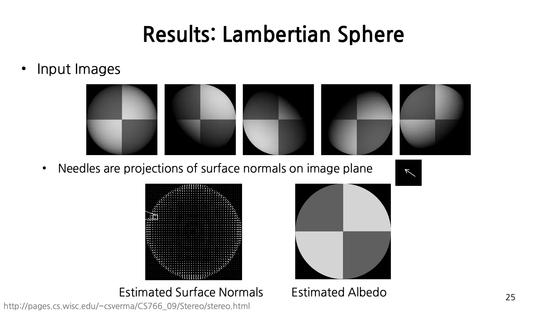
•
광원을 돌려가며 5장의 사진을 찍으면, 모든 점에 대해서 Surface Normal 과 Albedo 를 측정할 수 있음.